![]()
![]()
This package is designed to help the user specify, run, and then visualize and analyze the results of Ixodidae (hard-bodied ticks) population dynamics models. Such models exist in the literature, but the source code to run them is not always available. We wanted to provide an easy way for these models to be written and shared.
Install the package from CRAN with:
install.packages("IxPopDyMod")Here we provide a series of examples to help others see how models are specified and better understand the structure of the package. The examples highlight:
These examples all use and modify preset model configurations. If you
wish to create a custom model configuration, see
?config().
We start with config_ex_1, a simple model configuration
that doesn’t consider infection, and that has four life stages:
egg, larva, nymph, and
adult. This config is already loaded with the
package, but as an example here is how the config is
specified in R.
# library(IxPopDyMod)
devtools::load_all()
config_ex_1 <- config(
  cycle = life_cycle(
    transition("egg", "larva", function(a) a, transition_type = "probability", parameters = c(a = 1)),
    transition("egg", NULL, function(a) a, transition_type = "probability", mortality_type = "per_day", parameters = c(a = 0)),
    transition("larva", "nymph", function(a) a, transition_type = "probability", parameters = c(a = 0.01)),
    transition("larva", NULL, function(a) a, transition_type = "probability", mortality_type = "per_day", parameters = c(a = 0.99)),
    transition("nymph", "adult", function(a) a, transition_type = "probability", parameters = c(a = 0.1)),
    transition("nymph", NULL, function(a) a, transition_type = "probability", mortality_type = "per_day", parameters = c(a = 0.9)),
    transition("adult", "egg", function(a) a, transition_type = "probability", parameters = c(a = 1000)),
    transition("adult", NULL, function(a) a, transition_type = "probability", mortality_type = "per_day", parameters = c(a = 0))
  ),
  initial_population = c("adult" = 1000),
  steps = 29L
)
Here each transition is a probability rather than
duration (see below) and there are not predictors (like
temperature or the host community). All eggs hatch to larvae, 1% of
larvae make it to nymphs, 10% of nymphs become adults, and than each
adult lays 1000 eggs. The model starts with 1000 adults and runs for 29
time steps.
We give a new range of parameter values for number of eggs laid.
cfg1 <- config_ex_1
cfg2 <- config_ex_1
cfg3 <- config_ex_1

cfg1$cycle[[7]]$parameters[['a']] <- 800
cfg2$cycle[[7]]$parameters[['a']] <- 1000
cfg3$cycle[[7]]$parameters[['a']] <- 1200

modified_configs <- list(cfg1, cfg2, cfg3)
This gives us a list of three modified model configs,
which differ only in the number of eggs laid.
outputs <- lapply(modified_configs, run)The model output is a data frame where the column day
indicates Julian date, stage indicates tick life stage, and
pop is population size.
sapply(outputs, growth_rate)
#> [1] 0.9457416 1.0000000 1.0466351
growth_rate() calculates the multiplicative growth rate
for a model output. The population is stable with 1000 eggs laid, as
indicated by the growth rate 1. The population decreases
with 800 eggs laid, and increases with 1200 eggs laid.
temp_example_config$cycle
#> ** A life cycle
#> ** Number of transitions: 15
#> ** Unique life stages: __e, q_l, e_l, q_n, e_n, q_a, e_a, r_a
#> 1. __e -> q_l
#> 2. __e -> mortality
#> 3. q_l -> e_l
#> 4. q_l -> mortality
#> 5. e_l -> q_n
#> 6. e_l -> mortality
#> 7. q_n -> e_n
#> 8. q_n -> mortality
#> 9. e_n -> q_a
#> 10. e_n -> mortality
#> ... and 5 more transitions
Calling the life_cycle element in a config
gives a summary of the life cycle. Here we see the life stages, how many
transitions between life stages there are, and the first 10 transitions
are shown. Each transition is stored in the life_cycle as a
list, so they can be called using list indexing.
temp_example_config$cycle[[1]]
#> ** A transition
#> ** __e -> q_l
#> Transition type: duration
#> Predictors: x = list(pred = "temp", first_day_only = FALSE)
#> Parameters: a = 2.92e-05, b = 2.27
#> Function: (x, a, b) ifelse(x > 0, a * x^b, 0)
Here is the first transition from __e, eggs, to
q_l, questing larvae. This transition is a duration, so we
interpret the output as the rate at which it happens on the probability
with which it happens. It has a predictor, temperature. So the time to
transition from egg to questing larva is a temperature dependent
function. The parameters and function show this rate is
2.92e-05 * temp^2.27.
Here we highlight how this temperature dependence affects the output
of the model. We make a second config in which the daily
temperature is one degree warmer.
output <- run(temp_example_config)

# Predictor data for this example config is the temperature data from the Ogden config
# (host density data is dropped).
temp_pred2 <- readr::read_csv("./data-raw/ogden2005/predictors.csv") %>% dplyr::filter(pred == "temp")

temp_pred2$value <- temp_pred2$value + 1

temp_example_config2 <- temp_example_config
temp_example_config2$preds <- temp_pred2

output2 <- run(temp_example_config2)
Finally, we compare the outputs for a commonly measured aspect of tick populations, the number of questing nymphs.
output_qn <- subset(output, stage == 'q_n')
output2_qn <- subset(output2, stage == 'q_n')

plot(output2_qn$day, output2_qn$pop, type = 'l', col = 'red', lwd = 2, xlab = 'Day', ylab='Questing nymphs')
lines(output_qn$day, output_qn$pop, type = 'l', col = 'blue', lwd = 2)
Here you can see nymphs start questing earlier and reach a higher population in the warmer climate.
In the previous example there was no host community explicitly stated
and ticks had a constant probability of transition between life stages
(e.g., from larva to nymph). It is possible to instead model these
probabilities based on host community composition. Here transition from
questing larvae, q_l, to engorged larvae, e_l,
depends on the host_den, which is how the host community is
included in the transition.
host_example_config$cycle[[3]]
#> ** A transition
#> ** q_l -> e_l
#> Transition type: probability
#> Predictors: x = list(pred = "host_den", first_day_only = TRUE)
#> Parameters: a = 0.01, pref = c(deer = 0.25, mouse = 1, squirrel = 0.25), feed_success = c(deer = 0.49, mouse = 0.49, squirrel = 0.17)
#> Function: (x, a, pref, feed_success) {    if (length(pref)%%length(x) != 0) {        print(paste("error in find_n_feed, x:", length(x), "pref:",             length(pref)))    }    (1 - (1 - a)^(sum(x * pref)/sum(pref))) * sum(x * pref *         feed_success/sum(x * pref))}
This transition from questing larvae to engorged larvae depends on
host_den, host densities. Here some parameters in the
transition function have different values for each host species. Here
pref is larval preference for different host species and
feed_success is the probability an attached larva feeds to
completion on each host species.
In this example the temperature and host community are constant through time, but the package also supports variable temperature and host community data to see how seasonal or year-to-year variation in affects tick populations.
We now compare how different host densities affect tick populations. Here we vary the deer density.
cfg_lowdeer <- host_example_config
cfg_highdeer <- host_example_config

cfg_lowdeer$preds$value[cfg_lowdeer$preds$pred_subcategory == 'deer'] <- 0.1
cfg_highdeer$preds$value[cfg_highdeer$preds$pred_subcategory == 'deer'] <- 5

output_lowdeer <- run(cfg_lowdeer)
output_middeer <- run(host_example_config)
output_highdeer <- run(cfg_highdeer)

output_lowdeer_qn <- subset(output_lowdeer, stage == 'q_n')
output_middeer_qn <- subset(output_middeer, stage == 'q_n')
output_highdeer_qn <- subset(output_highdeer, stage == 'q_n')


plot(output_highdeer_qn$day, log10(output_highdeer_qn$pop), type = 'l', lwd = 2, col = '#1b9e77', yaxt = 'n', ylab ='Questing nymphs', xlab = 'Day', ylim = c(2,5))
lines(output_middeer_qn$day, log10(output_middeer_qn$pop), col = '#d95f02', lwd = 2)
lines(output_lowdeer_qn$day, log10(output_lowdeer_qn$pop), col = '#7570b3', lwd = 2)
text(x = 25, y = c(4.25,4,3.75), labels = c('High deer den.', 'Mid deer den.', 'Low deer den.'), col = c('#1b9e77', '#d95f02', '#7570b3'))
axis(side = 2, at = 2:5, labels = c(expression(10^2),expression(10^3),expression(10^4),expression(10^5)))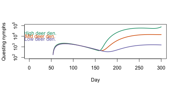
In the examples above we modeled a tick population without a tick-borne pathogen Here we give an example of how the package can be used to also include infection dynamics.
So far all examples have used transition functions loaded into the package, here we show how to define our own.
find_host <- function(x, y, a, pref) {
  1 - (1 - a)^sum(x * pref)
}infect_example_config$cycle
#> ** A life cycle
#> ** Number of transitions: 33
#> ** Unique life stages: __e, q_l, f_l, eil, eul, qin, qun, fun, fin, ein, eun, qia, qua, fua, fia, eia, eua, r_a
#> 1. __e -> q_l
#> 2. __e -> mortality
#> 3. q_l -> f_l
#> 4. q_l -> mortality
#> 5. f_l -> eil
#> 6. f_l -> eul
#> 7. eil -> qin
#> 8. eil -> mortality
#> 9. eul -> qun
#> 10. eul -> mortality
#> ... and 23 more transitionsHere we use the middle character of the life-stage key. It is either
i for infected or u for uninfected. We assume
no transovarial infection so questing larvae are uninfected. But after
they feed, f_l, they can either become engorged infected,
eil, or engorged uninfected, eul, larvae. This
is based on infect_fun, which as above has host
species-specific parameters of pref and
host_rc (reservoir competence).
Deer are important to the blacklegged tick as the main host of adult ticks. As such they are thought to increase tick populations (see above). But deer can also serve as hosts for juvenile tick life stages, and deer are poor reservoirs for Borrelia burgdorferi. So increased deer density may also decrease the proportion of bloodmeals juvenile ticks take from more competent reservoirs life mice. We use this simple model to illustrate this possibility.
deer_den <- c(0.1, 0.25, 0.5, 0.75, 1)
results_df <- data.frame(deer = deer_den, nymph_den = 0, nip = 0)

for (i in 1:5)
{
  cfg_mod <- infect_example_config
  cfg_mod$preds[1, 4] <- deer_den[i]
  out <- run(cfg_mod)


  results_df$nip[i] <- sum(out[out$stage=='qin','pop'])/(sum(out[out$stage=='qin','pop']) + sum(out[out$stage=='qun','pop']))

  results_df$nymph_den[i] <- sum(out[out$stage=='qin','pop']) + sum(out[out$stage=='qun','pop'])
}

plot(results_df$deer,results_df$nymph_den, xlab = 'Deer density', ylab = 'Number of questing nymphs')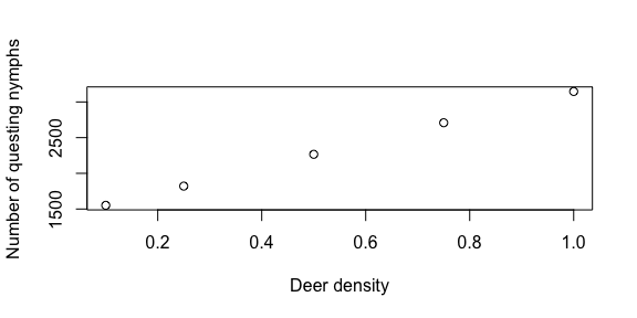
plot(results_df$deer,results_df$nip, xlab = 'Deer density', ylab = 'Nymph infection rate')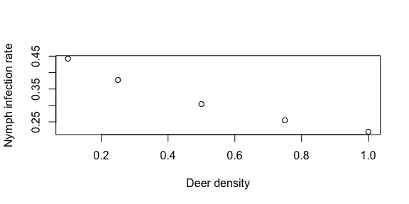
Here we see that as deer density increases the number of nymphs increases, but the nymph infection prevalence (NIP) goes down.