Vector Fields from Spatial Time Series of Population Abundance
Functions for converting time series of spatial abundance or density data in raster format to vector fields of population movement using the digital image correlation technique. More specifically, the functions in the package compute cross-covariance using discrete fast Fourier transforms for computational efficiency. Vectors in vector fields point in the direction of highest two dimensional cross-covariance. The package has a novel implementation of the digital image correlation algorithm that is designed to detect persistent directional movement when image time series extend beyond a sequence of two raster images.
You can install the released version of ICvectorfields from CRAN with:
install.packages("ICvectorfields")You can install the released version of ICvectorfields from GitHub with:
install.packages("devtools")
devtools::install_github("goodsman/ICvectorfields")Here is a demonstration of how the functions in the ICvectorfields package estimate movement and how to produce a vector field using functions in the package.
library(ICvectorfields)
library(ggplot2)
library(ggnewscale)
library(metR)
library(terra)
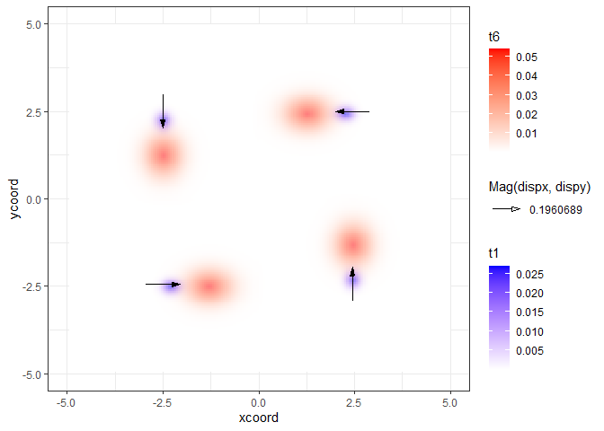
#> terra version 1.2.10One of the key advantages of the functions in ICvectorfields over other R software that uses cross-correlation or cross-covariance to estimate displacement is that the functions in ICvectorfields can estimate displacement in multiple, and opposing directions simultaneously. To demonstrate this capability a simulated data set was produced using a convection reaction equation, which is a partial differential equation with a diffusion term, an advection term for directed movement and a reaction term. Advection in the simulation was spatially variable: In the upper left quadrant of the spatial domain, advection was to the bottom of the domain, in the lower left quadrant, advection was to the right, in the lower right quadrant, advection was toward the top of the domain, and in the upper right quadrant, advection was to the left (see figure below). In all cases the speed of advection was 0.2 spatial units per unit time.
# import simulated data
data(SimData, package = "ICvectorfields")

# convert to raster stack
SimStack <- ICvectorfields::RastStackData(SimData)

# confirming dimension
dim(SimStack)
#> [1] 203 203   6
Because speed is constant in the simulation model, the DispFieldST function is appropriate for estimating orthogonal velocity vectors:
VFdf2 <- DispFieldST(SimStack, lag1 = 1, factv1 = 101, facth1 = 101, restricted = TRUE)
VFdf2
#>   rowcent colcent frowmin frowmax fcolmin fcolmax     centx     centy
#> 1      51      51       1     101       1     101 -2.499878  2.499878
#> 2     152      51     102     202       1     101 -2.499878 -2.450861
#> 3      51     152       1     101     102     202  2.450861  2.499878
#> 4     152     152     102     202     102     202  2.450861 -2.450861
#>        dispx      dispy
#> 1  0.0000000 -0.1960689
#> 2  0.1960689  0.0000000
#> 3 -0.1960689  0.0000000
#> 4  0.0000000  0.1960689
The movement speed is estimated as 0.196 units of space per unit time in each of the quadrants and the directions are consistent with simulated advection directions. Note that in the function above, the logical restricted argument is set to TRUE, whereas the default is FALSE. The restricted argument restricts the search for cross-covariance to areas within each of the grids that are designated using the factv1, and facth1 arguments to the function when set to TRUE. When restricted is set to false the algorithm searches the entire spatial domain to look for maximum cross-covariance. The estimated speed is a little under the simulated advection speed of 0.2 spatial units per unit time in all directions. The bias in the estimate is likely due to the diffusion term in the partial differential equation as diffusion obfuscates the impact of advection.
To plot vector fields produced by functions in ICvectorfields one can use ggplot2, and its extensions in the metR, and ggnewscale packages:
SimVF = ggplot() +
  xlim(c(-5, 5)) +
  ylim(c(-5, 5)) +
  geom_raster(data = SimData,
              aes(x = xcoord, y = ycoord, fill = t1)) +
  scale_fill_gradient(low = "white", high = "blue", na.value = NA) +
  new_scale("fill") +
  geom_raster(data = SimData,
              aes(x = xcoord, y = ycoord, fill = t6), alpha = 0.5) +
  scale_fill_gradient(low = "white", high = "red", na.value = NA) +
  geom_vector(data = VFdf2,
              aes(x = centx, y = centy,
                  mag = Mag(dispx, dispy),
                  angle = Angle(dispx, dispy))) +
  theme_bw()
SimVF
#> Warning: Removed 403 rows containing missing values (geom_raster).

#> Warning: Removed 403 rows containing missing values (geom_raster).