![]()
EcoNetGen lets you randomly generate a wide range of
interaction networks with specified size, average degree, modularity,
and topological structure. You can also sample nodes and links from
within simulated networks randomly, by degree, by module, or by
abundance. Simulations and sampling routines are implemented in FORTRAN,
providing efficient generation times even for large networks. Basic
visualization methods also included. Algorithms implemented here are
described in de Aguiar et al. (2017) arXiv:1708.01242.
EcoNetGen is now on CRAN and can be installed in the
usual way:
install.packages("EcoNetGen")See NEWS for a list of the most recent changes
to the development version and current CRAN release. You can install the
current development version of EcoNetGen from GitHub
with:
# install.packages("devtools")
devtools::install_github("cboettig/EcoNetGen")
This way requires you have a recent FORTRAN compiler available on your machine.
This is a basic example which generates a network. See
?netgen for documentation describing the parameter
arguments. Setting verbose = FALSE (default) suppresses the
output summary message.
library(EcoNetGen)
set.seed(123456) # for a reproducible simulation

network <- netgen(net_size = 150,
                  ave_module_size = 20,
                  min_module_size = 10,
                  min_submod_size = 5,
                  net_type = "bi-partite nested",
                  ave_degree = 10,
                  verbose = TRUE
                  )
#>
#> module count = 8
#> average degree = 6.10666666666667
#> average module size = 18.75
#> number of components = 1
#> size of largest component = 150
We can plot the resulting igraph as an adjacency
matrix:
adj_plot(network)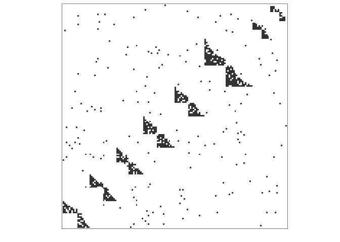
Network igraph objects can also be plotted using the
standard igraph plotting routines, for example:
library(igraph)
plot(network, vertex.size= 0, vertex.label=NA,
     edge.color = rgb(.22,0,1,.02), vertex.shape="none",
     edge.curved =TRUE, layout = layout_with_kk)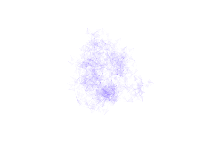
set.seed(123456) # for a reproducible random sampling
sampled <- netsampler(network,
                     key_nodes_sampler = "degree",
                     neighbors_sampler = "random",
                     n_key_nodes = 50,
                     n_neighbors = 0.5 # 50%
                    )
We can plot the adjacency network, coloring red the sampled nodes.
Note that adj_plot objects are just ggplot
graphs (geom_raster) under the hood, and can be modified
with the usual ggplot arguments, such as adding a title and
changing the color theme here.
library(ggplot2) # needed to modify plot

adj_plot(sampled) +
  ggtitle("Adjacency matrix of sampled vs full network") +
  scale_fill_manual(values = c("#ED4E33", "#3B7EA1"))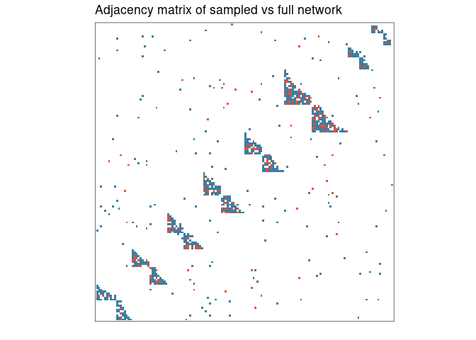
Don’t forget to check out the ggraph package, which
isn’t required for EcoNetGen but provides a lot of
additional great ways to plot your network. Here we plot the simulated
network color-coding the sampled nodes and edges (indicated by the label
“sampled” on vertices and edges):
library(ggraph)
ggraph(sampled, layout = 'kk') +
        geom_edge_link(aes(color = label), alpha=0.4) +
        geom_node_point(aes(color = label)) +
        theme_graph() +
        scale_color_manual(values = c("#ED4E33", "#3B7EA1")) +
        scale_edge_color_manual(values = c("#ED4E33", "#3B7EA1"))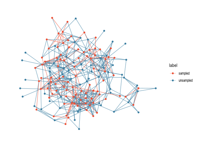
Or extract and plot just the sampled network:
subnet <- subgraph.edges(sampled,
                         E(sampled)[label=="sampled"])

ggraph(subnet, layout = 'graphopt') +
        geom_edge_link(alpha=0.4) +
        geom_node_point() +
theme_graph() 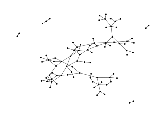
And we can compute common statistics from igraph as
well. Here we confirm that clustering by “edge betweeness” gives us the
expected number of modules:
community <- cluster_edge_betweenness(as.undirected(network))
length(groups(community))
#> [1] 8
We can check the size of each module as well:
module_sizes <- sizes(community)
module_sizes
#> Community sizes
#>  1  2  3  4  5  6  7  8
#> 18 18 19 22 19 32 11 11
Average degree:
mean(degree(as.undirected(network)))
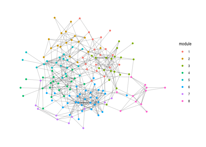
#> [1] 6.12We can also label and plot the cluster membership:
V(sampled)$module <- as.character(membership(community))ggraph(sampled, layout = 'kk') +
geom_edge_link(alpha=0.1) +
geom_node_point(aes(colour = module)) +
theme_graph()