
The aim of this package is to study directed dynamic functional connectivity in functional MRI. Dynamic graphical models (DGM) belong to the family of Dynamic Bayesian Networks. DGM is a collection of Dynamic Linear Models (DLM) [1], a dynamic multiple regression at each node. Moreover, DGM searches through all possible parent models and provides an interpretable fit in terms of regression model for each network node. There is a special variant of DGM called Multiregression Dynamic Models (MDM) which constrain the network to a acyclic graph [2,3], but with DGM, we do not use this constrain.
Current research aims to fully characterize DGM using simulations and big data from the Human Connectome Project (HCP) in order to test validity and reliability to make this new method available for neuroimaging research.
Schwab, S., Harbord, R., Zerbi, V., Elliott, L., Afyouni, S., Smith, J. Q., … Nichols, T. E. (2018). Directed functional connectivity using dynamic graphical models. NeuroImage. doi:10.1016/j.neuroimage.2018.03.074.
The installation is 2MB, with dependencies approx. 86MB.
install.packages("DGM")Before installing DGM and all it dependencies sometimes you have to upgrade the C++ compiler on the cluster scl enable devtoolset-4 bash
install.packages("devtools")
library(devtools)
install_github("schw4b/DGM", ref = "develop")We load simulation data of a 5-node network with 200 samples (time points) of one subject. Time series should already be mean centered.
library(DGM)
data("utestdata")
dim(myts)
[1] 200   5
Now, let’s do a full search across all possible parent models of the size n2(n-1). Here, with n=5, we have 16 possible models for each node, for example for node 3.
result=exhaustive.search(myts,3)
result$model.store
          [,1]      [,2]      [,3]      [,4]      [,5]      [,6]     [,7]      [,8]      [,9]     [,10]     [,11]     [,12]     [,13]     [,14]     [,15]     [,16]
[1,]    1.0000    2.0000    3.0000    4.0000    5.0000    6.0000    7.000    8.0000    9.0000   10.0000   11.0000   12.0000   13.0000   14.0000   15.0000   16.0000
[2,]    0.0000    1.0000    2.0000    4.0000    5.0000    1.0000    1.000    1.0000    2.0000    2.0000    4.0000    1.0000    1.0000    1.0000    2.0000    1.0000
[3,]    0.0000    0.0000    0.0000    0.0000    0.0000    2.0000    4.000    5.0000    4.0000    5.0000    5.0000    2.0000    2.0000    4.0000    4.0000    2.0000
[4,]    0.0000    0.0000    0.0000    0.0000    0.0000    0.0000    0.000    0.0000    0.0000    0.0000    0.0000    4.0000    5.0000    5.0000    5.0000    4.0000
[5,]    0.0000    0.0000    0.0000    0.0000    0.0000    0.0000    0.000    0.0000    0.0000    0.0000    0.0000    0.0000    0.0000    0.0000    0.0000    5.0000
[6,] -353.6734 -348.1476 -329.9119 -359.3472 -346.9735 -348.4044 -355.495 -347.4541 -337.3578 -333.6073 -353.8772 -349.6878 -346.9843 -358.2056 -341.7462 -355.5821
[7,]    0.5000    0.7300    0.6800    0.7700    0.7600    0.7800    0.800    0.7900    0.7300    0.7700    0.8100    0.7900    0.8300    0.8400    0.7800    0.8300
The columns are the 16 different models. First row indicates model number, rows 2-5 the parents, row 6 the model evidence, a log likelihood, and row 7 the discount factor delta, reflecting the smoothness of the time-varying regression coefficient (theta). To get the winning model, we simply maximize across model evidence.
which.max(result$model.store[6,])
[1] 3
Model number 3 with node 2 as a parent is most likely.
We do a full search on the subject level (exhautive search on each
node). The list returned contains all the models (models),
the winning models (winner), the adjacency matrix of the
network (adj).
s=subject(myts)
names(s)
[1] "models" "winner" "adj"
The adj structure contains the adjacency matrix of the
network (am), the model evidence (lpl), and
the discount factors delta (df).
names(s$adj)
[1] "am" "lpl" "df"The full network structure can be plotted as follows:
gplotMat(s$adj$am, hasColMap = F, title = "network")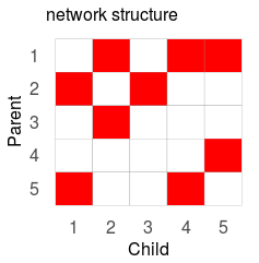
Estimates for a time-series with 1200 samples with a 2.6GHz CPU. 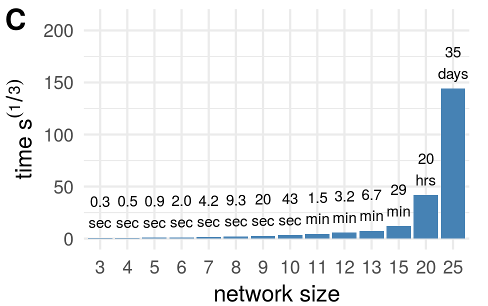
Timings are for one node only. To estimate the full network (all parents of all the nodes, the numbers above have to be multiplied by the number of nodes.
The greedy search, a network discovery optimization, is now available since DGM version 1.7 that can estimate 100-200 nodes within less than a day.