The primary goal of DEBBI (short for ‘Differential Evolution-based Bayesian Inference’) is to provide efficient access to and enable reproducible use of Bayesian inference algorithms such as Differential Evolution Markov Chain Monte Carlo, Differential Evolution Variation Inference, and Differential Evolution maximum a posteriori estimation. The second goal of this package is to be compatible with likelihood-free Bayesian inference methodologies that use approximations of the likelihood function such as probability density approximation, kernel-based approximate Bayesian computation, and synthetic likelihood.
You can install the development version of DEBBI from GitHub with:
# install.packages("devtools")
devtools::install_github("bmgaldo/DEBBI")Estimate mean parameters of two independent normal distributions with known standard deviations using DEMCMC
set.seed(43210)
library(DEBBI)
# simulate from model
dataExample=matrix(rnorm(100,c(-1,1),c(1,1)),nrow=50,ncol=2,byrow = T)
# list parameter names
param_names_example=c("mu_1","mu_2")
# log posterior likelihood function = log likelihood + log prior | returns a scalar
LogPostLikeExample=function(x,data,param_names){
out=0
names(x)<-param_names
# log prior
out=out+sum(dnorm(x["mu_1"],0,sd=1,log=T))
out=out+sum(dnorm(x["mu_2"],0,sd=1,log=T))
# log likelihoods
out=out+sum(dnorm(data[,1],x["mu_1"],sd=1,log=T))
out=out+sum(dnorm(data[,2],x["mu_2"],sd=1,log=T))
return(out)
}
# Sample from posterior
post <- DEMCMC(LogPostLike=LogPostLikeExample,
control_params=AlgoParamsDEMCMC(n_params=length(param_names_example),
n_iter=500,
n_chains=12,
burnin=100,
parallel_type = 'FORK',
n_cores_use = 4),
data=dataExample,
param_names = param_names_example)
#> initalizing chains...
#> 1 / 12
#> 2 / 12
#> 3 / 12
#> 4 / 12
#> 5 / 12
#> 6 / 12
#> 7 / 12
#> 8 / 12
#> 9 / 12
#> 10 / 12
#> 11 / 12
#> 12 / 12
#> chain initialization complete :)
#> initalizing FORK cluser with 4 cores
#> running DEMCMC
#> iter 100/500
#> iter 200/500
#> iter 300/500
#> iter 400/500
#> iter 500/500
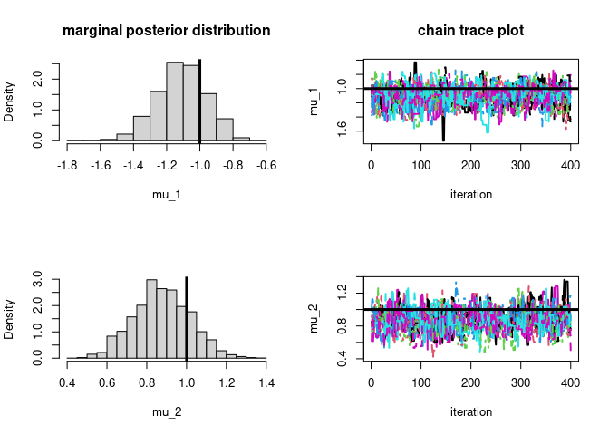
par(mfrow=c(2,2))
hist(post$samples[,,1],main="marginal posterior distribution",
xlab=param_names_example[1],prob=T)
# plot true parameter value as vertical line
abline(v=-1,lwd=3)
matplot(post$samples[,,1],type='l',ylab=param_names_example[1],
main="chain trace plot",xlab="iteration",lwd=2)
# plot true parameter value as horizontal line
abline(h=-1,lwd=3)
hist(post$samples[,,2],xlab=param_names_example[2],prob=T,main="")
# plot true parameter value as vertical line
abline(v=1,lwd=3)
matplot(post$samples[,,2],type='l',ylab=param_names_example[2],xlab="iteration",lwd=2)
# plot true parameter value as horizontal line
abline(h=1,lwd=3)
# let's check if the approximation is of good quality
#### mu_1
#### DEMCMC solution
# posterior mean
round(mean(post$samples[,,1]),3)
#> [1] -1.11
# posterior var
round(var(as.numeric(post$samples[,,1])),3)
#> [1] 0.022

#### Analytic solution (conjugate posteriors)
# posterior mean
round(1/(1+50/1)*(sum(dataExample[,1])),3)
#> [1] -1.101
# posterior var
round(1/(1+50/1),3)
#> [1] 0.02

#### mu_2
# posterior mean  (conjugate posteriors)
round(mean(post$samples[,,2]),3)
#> [1] 0.875
# posterior var
round(var(as.numeric(post$samples[,,2])),3)
#> [1] 0.02

#### Analytic solution
# posterior mean
round(1/(1+50/1)*(sum(dataExample[,2])),3)
#> [1] 0.876
# posterior var
round(1/(1+50/1),3)
#> [1] 0.02Find posterior mode (a.k.a. maximum a posteriori or MAP) of mean parameters of two independent normal distributions with known standard deviations using DE
# optimize posterior wrt to theta
map <- DEMAP(LogPostLike=LogPostLikeExample,
             control_params=AlgoParamsDEMAP(n_params=length(param_names_example),
                                            n_iter=100,
                                            n_chains=12,
                                            return_trace = T,
                                            parallel_type = 'FORK',
                                            n_cores_use = 4),
             data=dataExample,
             param_names = param_names_example)
#> initalizing chains...
#> 1 / 12
#> 2 / 12
#> 3 / 12
#> 4 / 12
#> 5 / 12
#> 6 / 12
#> 7 / 12
#> 8 / 12
#> 9 / 12
#> 10 / 12
#> 11 / 12
#> 12 / 12
#> chain initialization complete  :)
#> initalizing FORK cluser with 4 cores
#> running DE to find MAP
#> iter 100/100


par(mfrow=c(2,2))

# plot particle trace plot for mu 1
matplot(map$theta_trace[,,1],type='l',ylab=param_names_example[1],xlab="iteration",lwd=2)
# plot true parameter value as horizontal line
abline(h=-1,lwd=3)

# plot particle trace plot for mu 2
matplot(map$theta_trace[,,2],type='l',ylab=param_names_example[2],xlab="iteration",lwd=2)
# plot true parameter value as horizontal line
abline(h=1,lwd=3)

matplot(map$log_post_like_trace,type='l',ylab='log posterior likelihood',xlab="iteration",lwd=2)
abline(h=-1,lwd=3)


# let's check if the approximation is of good quality
#### mu_1
#### DEMAPsolution
# posterior mode
round(map$map_est[1],3)
#> [1] -1.101

#### Analytic solution (conjugate posteriors)
# posterior mode
round(1/(1+50/1)*(sum(dataExample[,1])),3)
#> [1] -1.101

#### mu_2
#### DEMAP solution
# posterior mode
round(map$map_est[2],3)
#> [1] 0.876

#### Analytic solution (conjugate posteriors)
# posterior mode
round(1/(1+50/1)*(sum(dataExample[,2])),3)
#> [1] 0.876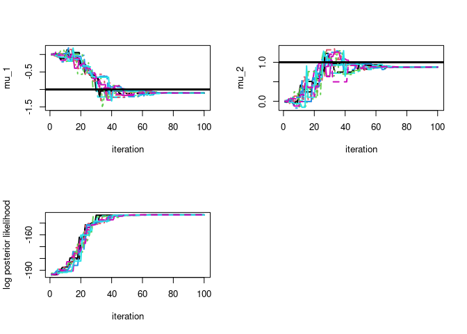
Optimize parameters lambda of Q(theta|lambda) to minimize the KL Divergence (maximize the ELBO) between Q and the likelihood*prior
# optimize KL between approximating distribution Q (mean-field approximation) and posterior
vb <- DEVI(LogPostLike=LogPostLikeExample,
           control_params=AlgoParamsDEVI(n_params=length(param_names_example),
                                         n_iter=200,
                                         n_samples_ELBO = 5,
                                         n_chains=12,
                                         use_QMC = F,
                                         n_samples_LRVB = 25,
                                         purify=10,
                                         return_trace = T,
                                            parallel_type = 'FORK',
                                            n_cores_use = 4),
           data=dataExample,
           param_names = param_names_example)
#> initalizing chains...
#> 1 / 12
#> 2 / 12
#> 3 / 12
#> 4 / 12
#> 5 / 12
#> 6 / 12
#> 7 / 12
#> 8 / 12
#> 9 / 12
#> 10 / 12
#> 11 / 12
#> 12 / 12
#> chain initialization complete  :)
#> initalizing FORK cluser with 4 cores
#> running DE to find best variational approximation
#> iter 100/200
#> iter 200/200
#> Attemtping LRVB covariance correction.
#> LRVB correction was a success!


par(mfrow=c(2,2))

# plot particle trace plot for mu 1
matplot(vb$lambda_trace[,,1],type='l',ylab=paste0(param_names_example[1]," mean"),xlab="iteration",lwd=2)
matplot(vb$lambda_trace[,,2],type='l',ylab=paste0(param_names_example[2]," mean"),xlab="iteration",lwd=2)

matplot(vb$lambda_trace[,,3],type='l',ylab=paste0(param_names_example[1]," log sd"),xlab="iteration",lwd=2)
matplot(vb$lambda_trace[,,4],type='l',ylab=paste0(param_names_example[2]," log sd"),xlab="iteration",lwd=2)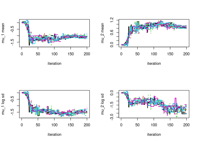
par(mfrow=c(1,1))
matplot(vb$ELBO_trace,type='l',ylab='ELBO',xlab="iteration",lwd=2)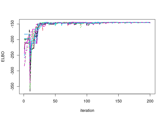
# let's check if the approximation is of good quality
#### DEVI solution
# posterior mean
round(vb$means,3)
#> param_1_mean param_2_mean
#>        -0.97         0.92
# posterior covariance
round((vb$covariance),3)
#>      [,1] [,2]
#> [1,] 0.02 0.00
#> [2,] 0.00 0.02

#### Analytic solution (conjugate posteriors)
# posterior mean
round(c(1/(1+50/1)*(sum(dataExample[,1])),1/(1+50/1)*(sum(dataExample[,2]))),3)
#> [1] -1.101  0.876
# posterior covariance
diag(c(round(1/(1+50/1),3),
       round(1/(1+50/1),3)))
#>      [,1] [,2]
#> [1,] 0.02 0.00
#> [2,] 0.00 0.02