The DALSM R-package enables to fit a nonparametric double location-scale model to right- and interval-censored data, see Lambert (2021) for methodological details.
Consider a vector \((Y,\mathbf{z},\mathbf{x})\) where \(Y\) is a univariate continuous response, \(\mathbf{z}\) a p-vector of categorical covariates, and \(\mathbf{x}\) a J-vector of quantitative covariates. The response could be subject to right-censoring, in which case one only observes \((T,\Delta)\), where \(T=\min\{Y,C\}\), \(\Delta=I(Y\leq C)\) and \(C\) denotes the right-censoring value that we shall assume independent of \(Y\) given the covariates. The response could also be interval-censored, meaning that it is only known to lie within an interval \((Y^L,Y^U)\).
A location-scale model is considered to describe the distribution of the response conditionally on the covariates, \[Y = \mu(\mathbf{z},\mathbf{x}) + \sigma(\mathbf{z},\mathbf{x})\varepsilon\] where \(\mu(\mathbf{z},\mathbf{x})\) denotes the conditional location, \(\sigma(\mathbf{z},\mathbf{x})\) the conditional dispersion, and \(\varepsilon\) an error term independent of \(\mathbf{z}\) and \(\mathbf{x}\) with fixed first and second order moments, \(\mathrm{E}(\varepsilon)=0\) and \(\mathrm{V}(\varepsilon)=1\).
Assume that independent copies \((y_i,\mathbf{z}_ i,\mathbf{x}_ i)~(i=1,\ldots,n)\) are observed on \(n\) units with the possibility of right or interval-censoring on \(y_i\) as described above. Additive models for the conditional location and dispersion of the response are specified, \[\mu(z_i, x_i)= \beta_0+ \Sigma_ {k=1}^p \beta_k z_{ik}+\Sigma_ {j=1} ^{J} {f_j ^{\mu}}(x_ {ij})\] \[\log\sigma(z_i,x_i)= \delta_0+\Sigma_ {k=1}^p \delta_k z_ {ik}+\Sigma_ {j=1}^{J} {{f_{j}^{\sigma}}}(x_ {ij})\] where \(f_{j}^{\mu}(\cdot)\) and \(f_{j}^{\sigma}(\cdot)\) denote smooth additive terms quantifying the effect of the \(j {th}\) quantitative covariate on the conditional mean and dispersion. The additive terms in the conditional location and dispersion models can be approximated using linear combinations of (recentered) B-splines, \[f^ {\mu}_ j=\left(\Sigma_ {\ell=1}^L {b_ {j\ell}}(x_ {ij})\theta_ {\ell j}^\mu\right)_ {i=1}^n=\mathbf{B}_ j\pmb{\theta}_ j^\mu\] \[f^ {\sigma}_ j=\left(\Sigma_ {\ell=1}^L {b_ {j\ell}}(x_ {ij})\theta_ {\ell j}^\sigma\right)_ {i=1}^n = \mathbf{B}_ j\pmb{\theta}_ j^\sigma\] where \([\mathbf{B}_ j]_ {i\ell}={b_{ j\ell}}(x_ {ij})\).
Gaussian Markov random field (GMRF) priors penalizing changes in neighbour B-spline parameters are taken, \[p(\pmb{\theta}^ {\mu}_ {j}|\lambda_ j^\mu) \propto \exp\left( -{1\over 2}{\pmb{\theta}^ \mu_ j}^ \top (\lambda^ {\mu}_ j\mathbf{P}^ \mu) \pmb{\theta}^ \mu_ j \right)\] \[p(\pmb{\theta}^ {\sigma}_ {j}|\lambda_ j^\sigma) \propto \exp\left( -{1\over 2}{\pmb{\theta}^ \sigma_ j}^ \top (\lambda^ {\sigma}_ j\mathbf{P}^ \sigma) \pmb{\theta}^ \sigma_ j \right) \]
where \(\mathbf{P}^ \mu, \mathbf{P}^ \sigma\) are penalty matrices and \(\lambda^ {\mu}_ {j},\lambda^ {\sigma}_ {j}\) positive penalty parameters for the location and dispersion submodels, respectively. For penalty matrices of order 2, increasingly large values for these parameters point to linear effects for the additive terms.
The error term \(\varepsilon\) is assumed to have fixed first and second order moments, \(\mathrm{E}(\varepsilon)=0\) and \(\mathrm{V}(\varepsilon)=1\). To get away from the constraining and sometimes unrealistic normality hypothesis, a flexible form based on P-splines is indirectly assumed for the error density through the log of the hazard function. Lagrange multipliers are used to force mean and variance constraints. We refer to Section 2.5 and Algorithm 3 in Lambert (2021) for more details and to function densityLPS in the DALSM package for computational aspects to handle right- and interval-censored data.
Marginal posterior distributions of the penalty parameters in the error density and in the location and dispersion submodels are approximated by starting from the following identity, \[p(\pmb{\lambda} | {\cal D}) = {p(\pmb{\psi},\pmb{\lambda}|{\cal D}) \over p(\pmb{\psi}|\pmb{\lambda},{\cal D})}\] where \(\lambda\) and \(\pmb{\psi}\) generically denote the penalty and the penalized parameters. Thanks to the GMRF prior for \((\pmb{\psi}|\lambda)\), a Laplace approximation to the conditional posterior in the numerator is relevant. When that expression is evaluated at the conditional posterior mode \(\hat\psi_ \lambda\), one obtains the following approximation to the marginal posterior of the penalty parameters \[\tilde p (\pmb{\lambda} | {\cal D}) \propto p(\hat\psi_ \lambda, \pmb{\lambda} | {\cal D}) |\Sigma_ \lambda|^ {1/2}\]
where \(\Sigma_\lambda\) denotes the conditional variance-covariance matrix. The mode of \(\tilde{p}(\pmb{\lambda}|{\cal D})\) could be chosen if point values for the penalty parameters are desired. The combination of Bayesian P-splines with the preceding approximation to the marginal posterior of \(\pmb{\lambda}\) is shortly named Laplace P-splines.
Model fitting alternates the estimation of the regression and spline parameters in the location-scale model (see Algorithm 1 in Lambert 2021), the selection of the penalty parameters (see Algorithm 2) and the update of the error density (see Algorithm 3). The whole procedure is implemented in function DALSM of the package.
The data of interest come from the European Social Survey (ESS 2016) with a focus on the money available per person in Belgian households for respondents aged 25-55 when the main source of income comes from wages or salaries (\(n=756\)). Each person reports the total net monthly income of the household in one of 10 decile-based intervals: \(1: <1120\) \((n_1=8)\), \(2: [1120,1399]\) \((n_2=13)\), \(3: [1400,1719]\) \((n_3=47)\), \(4: [1720,2099]\) \((n_4=53)\), \(5: [2100,2519]\) \((n_5=82)\), \(6: [2520,3059]\) \((n_6=121)\), \(7: [3060,\) \(3739]\) \((n_7=167)\), \(8:[3740,4529]\) \((n_8=126)\), \(9: [4530,5579]\) \((n_9=74)\), \(10: \geq 5580\) euros \((n_{10}=65)\).
We model the relationship between disposable income per person (\(91.4\) percents interval-censored, \(8.6\) percents right-censored) and the availability of (at least) two income (\(64.2\) percents) in the household, as well as the age (\(41.0\pm8.83\) years) and number of years of education completed (\(14.9\pm3.34\) years) by the respondent. This individualized income is obtained by dividing the household one by the OECD-modified equivalence (Hagenaars1994), as recommended by the Statistical Office of the European Union (EUROSTAT).
Let us load the package and visualize typical response values:
## Package installation from R-CRAN
## install.packages("DALSM")
## Alternatively, installation from GitHub:
## install.packages("devtools")
## devtools::install_github("plambertULiege/DALSM")

## Package loading
library(DALSM)

## Data reading
data(DALSM_IncomeData)
resp = DALSM_IncomeData[,1:2]
head(resp,20) ## Visualize first 20 censored income values
## inc.low inc.up
## 1 1.5300000 1.8700000
## 2 1.1333333 1.3851852
## 3 2.0400000 2.4933333
## 4 2.4933333 3.0200000
## 5 1.8120000 2.2320000
## 6 1.7200000 2.1000000
## 7 1.7200000 2.1000000
## 8 1.7200000 2.1000000
## 9 1.2240000 1.4960000
## 10 2.4933333 3.0200000
## 11 1.7200000 2.1000000
## 12 2.0777778 2.5166667
## 13 1.4000000 1.7000000
## 14 2.0400000 2.4933333
## 15 1.8120000 2.2320000
## 16 1.1666667 1.4000000
## 17 1.6800000 2.0400000
## 18 2.1571429 2.6571429
## 19 0.5384615 0.6615385
## 20 2.6571429 Infsummary(DALSM_IncomeData[,3:5]) ## Summary stats for covariates## twoincomes age eduyrs
## Min. :0.0000 Min. :25.00 Min. : 0.00
## 1st Qu.:0.0000 1st Qu.:34.00 1st Qu.:12.00
## Median :1.0000 Median :41.00 Median :15.00
## Mean :0.6415 Mean :41.03 Mean :14.88
## 3rd Qu.:1.0000 3rd Qu.:49.00 3rd Qu.:17.00
## Max. :1.0000 Max. :55.00 Max. :26.00Most reported income values (in thousand euros) are interval-censored (with finite values for the upper bound of the interval), some are right-censored (with an Inf value for the upper bound of the interval) for respondents belonging to households whose net monthly income exceeds the last decile.
The nonparametric double location-scale model (with additive age and eduyrs terms and a fixed effect for the twoincomes indicator can be fitted using the DALSM function:
fit = DALSM(y=resp,
           formula1 = ~twoincomes+s(age)+s(eduyrs),
           formula2 = ~twoincomes+s(age)+s(eduyrs),
           data = DALSM_IncomeData)
print(fit)
## -----------------------------------------------------------------------
## Double Additive Location-SCALE Model
## -----------------------------------------------------------------------
## Fixed effects for Location:
## est se low up Z Pval
## (Intercept) 1.572 0.062 1.450 1.695 25.234 0
## twoincomes 0.252 0.051 0.152 0.352 4.957 0
##
## 2 additive term(s) in Location: Eff.dim / Test No effect
## ED.hat low up Chi2 Pval
## age 4.247 2.277 4.977 13.839 0.01
## eduyrs 3.554 1.811 4.679 118.901 0.00
##
## Fixed effects for Dispersion:
## est se low up Z Pval
## (Intercept) -0.436 0.086 -0.604 -0.268 -5.092 0.000
## twoincomes -0.042 0.070 -0.179 0.094 -0.610 0.542
##
## 2 additive term(s) in Dispersion: Eff.dim / Test No effect
## ED.hat low up Chi2 Pval
## age 3.318 1.456 4.409 15.249 0.002
## eduyrs 3.311 1.508 4.329 41.345 0.000
##
## 10 B-splines per additive component in location
## 10 B-splines per additive component in dispersion
## 20 B-splines for the error density on (-3.76,6.64)
##
## Total sample size: 756 ; Credible level for CI: 0.95
## Uncensored data: 0 (0 percents)
## Interval Censored data: 691 (91.4 percents)
## Right censored data: 65 (8.6 percents)
## -----------------------------------------------------------------------
## Convergence status: TRUE
## Elapsed time: 0.7 seconds (5 iterations)
## -----------------------------------------------------------------------It suggests an average increase of 252 euros (available per person in
the household) when the respondent and his/her partner are in paid work
(conditionally on Age and Educ), while the effect on
dispersion is not statistically significant.
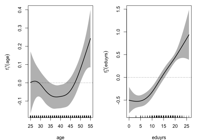
The effects of Age and Educ on the conditional mean
and dispersion can be visualized on the plots below with the estimated
additive terms.
plot(fit, new.dev=FALSE)
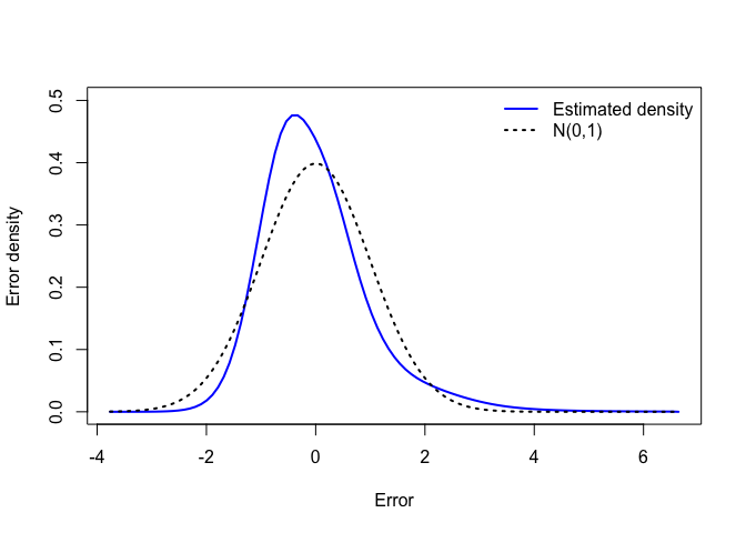
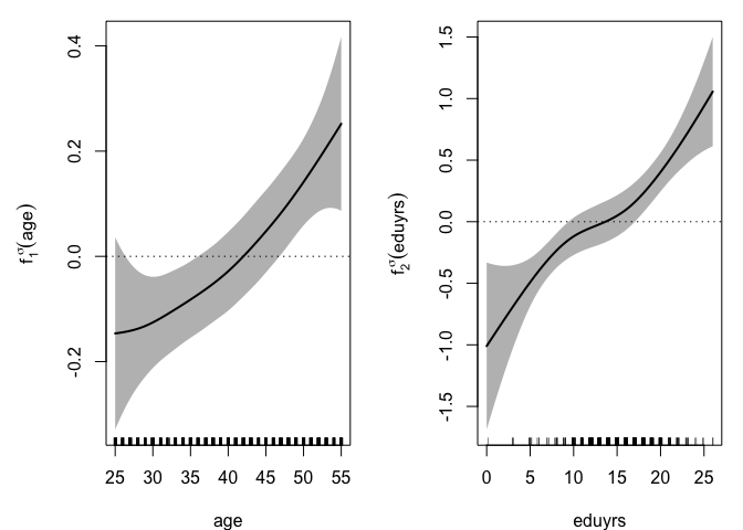
The amount of money available per person in the household tends to decrease with age, see \(f_1^\mu(\mathrm{age})\), between approximately 27 and 37 (most likely due the arrival of children in the family) and to increase after 40 (probably thanks to wage increase with seniority and the departure of children). The log-dispersion significantly increases with Age, see \(f_1^\sigma(\mathrm{age})\), with an acceleration over 30. However, the dominant effect comes from the respondent’s level of education, with a difference of about 1,000 euros (in expected disposable income per person) between a less educated (6 years) and a highly educated (20 years) respondent, see \(f_2^\mu(\mathrm{eduyrs})\). The effect on dispersion is also large, see \(f_2^\sigma(\mathrm{eduyrs})\), with essentially an important contrast between less and highly educated respondents, the latter group showing the largest heterogeneity. The estimated density for the error term can also be seen, with a right-skewed shape clearly distinguishable from the Gaussian one often implicitly assumed when fitting location-scale regression models.
Besides fitting Nonparametric Double Additive Location-Scale Model to censored data, the DALSM package contains an independent and very fast function, densityLPS, for density estimation from right- or interval-censored data with possible constraints on the mean and variance using Laplace P-splines.
Let us generate interval-censored (IC) data from a Gamma(10,2) distribution with mean 5.0 and variance 2.5. The mean width of the simulated IC intervals is 2.0. Part of the data are also right-censored (RC) with RC values generated from an exponential distribution with mean 15.0.
## Generation of right- and interval-censored data
set.seed(123)
n = 500 ## Sample size
x = rgamma(n,10,2) ## Exact (unobserved) data
width = runif(n,1,3) ## Width of the IC data (mean width = 2)
w = runif(n) ## Positioning of the exact data within the interval
xmat = cbind(pmax(0,x-w*width),x+(1-w)*width) ## Generated IC data
t.cens = rexp(n,1/15) ## Right-censoring values
idx.RC = (1:n)[t.cens<x] ## Id's of the right-censored units
xmat[idx.RC,] = cbind(t.cens[idx.RC],Inf) ## Data for RC units: (t.cens,Inf)
head(xmat,15)
## [,1] [,2]
## [1,] 0.8279792 Inf
## [2,] 6.6526685 8.204466
## [3,] 1.1579633 Inf
## [4,] 4.1784981 6.277058
## [5,] 6.6143492 8.306603
## [6,] 3.7696512 5.799582
## [7,] 2.4766237 Inf
## [8,] 2.3888812 4.441426
## [9,] 5.9867783 7.392858
## [10,] 3.6321041 Inf
## [11,] 4.7570358 6.498024
## [12,] 4.3883940 5.995044
## [13,] 2.0614651 Inf
## [14,] 5.1459398 Inf
## [15,] 3.3849118 InfThe density can be estimated from the censored data using function densityLPS. Optionally, the mean and variance of the estimated density can also be forced to some fixed values, here 5.0 and 2.5, respectively. We also choose to force the left end of the distribution support to be 0:
## Density estimation from IC data
obj.data = Dens1d(xmat,ymin=0) ## Prepare the IC data for estimation
obj = densityLPS(obj.data, Mean0=10/2, Var0=10/4) ## Estimation with fixed mean and variance
print(obj)
## -----------------------------------------------------------------------
## Constrained Density/Hazard estimation from censored data using LPS
## -----------------------------------------------------------------------
## INPUT:
## Total sample size: 500
## Uncensored data: 0 (0 percents)
## Interval-censored (IC) data: 367 (73.4 percents)
## Right-censored (RC) data: 133 (26.6 percents)
## ---
## Range of the IC data: (0.1708629,12.56085)
## Range of the RC data: (0.009145886,7.785088)
## ---
## Assumed support: (0,14.69175)
## Number of small bins on the support: 501
## Number of B-splines: 25 ; Penalty order: 2
##
## OUTPUT:
## Returned functions: ddist, pdist, hdist, Hdist(x)
## Parameter estimates: phi, tau
## Value of the estimated cdf at +infty: 1
## Constraint on the Mean: 5 ; Fitted mean: 5
## Constraint on the Variance: 2.5 ; Fitted variance: 2.499669
## Selected penalty parameter <tau>: 22.5
## Effective number of parameters: 5.4
## -----------------------------------------------------------------------
## Elapsed time: 0.1 seconds (6 iterations)
## -----------------------------------------------------------------------The estimated density and cdf can also be visualized and compared to their ‘true’ Gamma(10,2) counterparts used to generate the data:
plot(obj) ## Plot the estimated density
curve(dgamma(x,10,2), ## ... and compare it to the true density (in red)
      add=TRUE,col="red",lwd=2,lty=2)
legend("topright",col=c("black","red"),lwd=c(2,2),lty=c(1,2),
        legend=c("Estimated density","True density"),bty="n")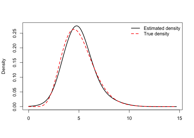
## Same story for the cdf
with(obj, curve(pdist(x),ymin,ymax,lwd=2,xlab="",ylab="F(x)"))
curve(pgamma(x,10,2),add=TRUE,col="red",lwd=2,lty=2)
legend("right",col=c("black","red"),lwd=c(2,2),lty=c(1,2),
        legend=c("Estimated cdf","True cdf"),bty="n")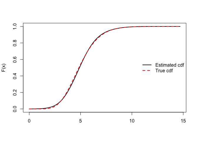
Estimated density (pdf), distribution (cdf), hazard and cumulative hazard functions are also directly available:
xvals = seq(2,10,by=2)
with(obj, cbind(x=xvals, fx=ddist(xvals), Fx=pdist(xvals),
                hx=hdist(xvals), Hx=Hdist(xvals)))
## x fx Fx hx Hx
## [1,] 2 0.031622032 0.01849226 0.03221816 0.01866538
## [2,] 4 0.234756524 0.26468056 0.31927749 0.30745026
## [3,] 6 0.186674735 0.76413790 0.79144393 1.44450795
## [4,] 8 0.037761707 0.95797288 0.89847167 3.16944027
## [5,] 10 0.006598059 0.99509435 1.34498959 5.31736848DALSM: Nonparametric Double Additive Location-Scale Model (DALSM). Copyright (C) 2021-2023 Philippe Lambert
This program is free software: you can redistribute it and/or modify it under the terms of the GNU General Public License as published by the Free Software Foundation, either version 3 of the License, or (at your option) any later version.
This program is distributed in the hope that it will be useful, but WITHOUT ANY WARRANTY; without even the implied warranty of MERCHANTABILITY or FITNESS FOR A PARTICULAR PURPOSE. See the GNU General Public License for more details.
You should have received a copy of the GNU General Public License along with this program. If not, see https://www.gnu.org/licenses/.
[1] Lambert, P. (2021) Fast Bayesian inference using Laplace approximations in nonparametric double additive location-scale models with right- and interval-censored data. Computational Statistics and Data Analysis, 161: 107250. doi:10.1016/j.csda.2021.107250
[2] Lambert, P. (2021) R-package DALSM (Nonparametric Double Additive Location-Scale Model)- R-cran ; GitHub: plambertULiege/DALSM