![]()
![]()
The goal of BeeGUTS is to analyse the survival toxicity tests performed for bee species. It can be used to fit a Toxicokinetic-Toxicodynamic (TKTD) model adapted for bee standard studies (acute oral, acute contact, and chronic oral studies). The TKTD model used is the General Unified Threshold model of Survival (GUTS).
The model is based on the following publications:
Baas, J., Goussen, B., Taenzler, V., Roeben, V., Miles, M., Preuss, T.G., van den Berg, S. and Roessink, I. (2024), Comparing Sensitivity of Different Bee Species to Pesticides: A TKTD modeling approach. Environ Toxicol Chem, 43: 1431-1441. https://doi.org/10.1002/etc.5871
Baas, J., Goussen, B., Miles, M., Preuss, T.G. and Roessink, I. (2022), BeeGUTS—A Toxicokinetic–Toxicodynamic Model for the Interpretation and Integration of Acute and Chronic Honey Bee Tests. Environ Toxicol Chem, 41: 2193-2201. https://doi.org/10.1002/etc.5423
Jager T, Albert C, Preuss TG, Ashauer R. General unified threshold model of survival–a toxicokinetic-toxicodynamic framework for ecotoxicology. Environ Sci Technol. 2011 Apr 1;45(7):2529-40. doi: 10.1021/es103092a. Epub 2011 Mar 2. PMID: 21366215.
You can install the released version of BeeGUTS from CRAN with:
install.packages("BeeGUTS")And the development version from GitHub with:
# install.packages("devtools")
devtools::install_github("ibacon-GmbH-Modelling/BeeGUTS")Detailed documentation is available here
This is a basic example which shows you how to solve a common problem:
library(BeeGUTS)
#> BeeGUTS (Version 1.5.0, packaged on the: )
#> - For execution on a local, multicore CPU with excess RAM we recommend calling
#>       options(mc.cores = parallel::detectCores()-1)
#> - In addition to the functions provided by 'BeeGUTS', we recommend using the packages:
#>    - 'bayesplot' for posterior analysis, model checking, and MCMC diagnostics.
#>    - 'loo' for leave-one-out cross-validation (LOO) using Pareto smoothed
#>        importance sampling (PSIS), comparison of predictive errors between models, and
#>        widely applicable information criterion (WAIC).
file_location <- system.file("extdata", "betacyfluthrin_chronic_ug.txt", package = "BeeGUTS") # Load the path to one of the example file
lsData <- dataGUTS(file_location = file_location, test_type = 'Chronic_Oral', cstConcCal = FALSE) # Read the example file
plot(lsData) # Plot the data
#> [[1]]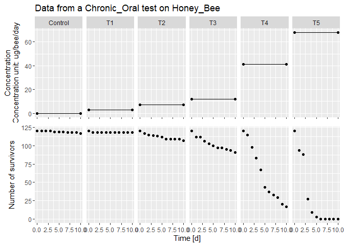
fit <- fitBeeGUTS(lsData, modelType = "SD", nIter = 3000, nChains = 1) # Fit a SD model. This can take some time...
#>
#> SAMPLING FOR MODEL 'GUTS_SD' NOW (CHAIN 1).
#> Chain 1:
#> Chain 1: Gradient evaluation took 0.00301 seconds
#> Chain 1: 1000 transitions using 10 leapfrog steps per transition would take 30.1 seconds.
#> Chain 1: Adjust your expectations accordingly!
#> Chain 1:
#> Chain 1:
#> Chain 1: Iteration:    1 / 3000 [  0%]  (Warmup)
#> Chain 1: Iteration:  300 / 3000 [ 10%]  (Warmup)
#> Chain 1: Iteration:  600 / 3000 [ 20%]  (Warmup)
#> Chain 1: Iteration:  900 / 3000 [ 30%]  (Warmup)
#> Chain 1: Iteration: 1200 / 3000 [ 40%]  (Warmup)
#> Chain 1: Iteration: 1500 / 3000 [ 50%]  (Warmup)
#> Chain 1: Iteration: 1501 / 3000 [ 50%]  (Sampling)
#> Chain 1: Iteration: 1800 / 3000 [ 60%]  (Sampling)
#> Chain 1: Iteration: 2100 / 3000 [ 70%]  (Sampling)
#> Chain 1: Iteration: 2400 / 3000 [ 80%]  (Sampling)
#> Chain 1: Iteration: 2700 / 3000 [ 90%]  (Sampling)
#> Chain 1: Iteration: 3000 / 3000 [100%]  (Sampling)
#> Chain 1:
#> Chain 1:  Elapsed Time: 101.544 seconds (Warm-up)
#> Chain 1:                165.025 seconds (Sampling)
#> Chain 1:                266.569 seconds (Total)
#> Chain 1:
#> Warning: Tail Effective Samples Size (ESS) is too low, indicating posterior variances and tail quantiles may be unreliable.
#> Running the chains for more iterations may help. See
#> https://mc-stan.org/misc/warnings.html#tail-ess
traceplot(fit) # Produce a diagnostic plot of the fit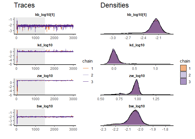
plot(fit) # Plot the fit results
#> [[1]]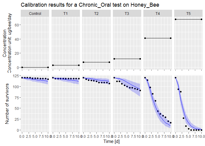
summary(fit) # Gives a summary of the results
#> Computing summary can take some time. Please be patient...Summary:
#>
#> Bayesian Inference performed with Stan.
#>  Model type: SD
#>  Bee species: Honey_Bee
#>
#>  MCMC sampling setup (select with '$setupMCMC')
#>  Iterations: 3000
#>  Warmup iterations: 1500
#>  Thinning interval: 1
#>  Number of chains: 1
#>
#> Priors of the parameters (quantiles) (select with '$Qpriors'):
#>
#>  parameters      median        Q2.5       Q97.5
#>          hb 8.32763e-03 1.09309e-04 6.34432e-01
#>          kd 2.62826e-03 1.17073e-06 5.90041e+00
#>          zw 8.24621e-03 1.19783e-06 5.67693e+01
#>          bw 1.84061e-03 1.69711e-06 1.99625e+00
#>
#> Posteriors of the parameters (quantiles) (select with '$Qposteriors'):
#>
#>  parameters      median        Q2.5       Q97.5
#>       hb[1] 6.73561e-03 1.98921e-03 1.00686e-02
#>  parameters      median        Q2.5       Q97.5
#>          kd 1.01806e+00 7.20743e-01 2.87306e+00
#>          zw 9.41747e+00 4.98442e+00 1.06524e+01
#>          bw 8.86067e-03 6.00886e-03 1.04942e-02
#>
#>
#>  Maximum Rhat computed (na.rm = TRUE): 1.034252
#>  Minimum Bulk_ESS: 120
#>  Minimum Tail_ESS: 73
#>  Bulk_ESS and Tail_ESS are crude measures of effecting sampling size for
#>       bulk and tail quantities respectively. An ESS > 100 per chain can be
#>       considered as a good indicator. Rhat is an indicator of chains convergence.
#>       A Rhat <= 1.05 is a good indicator of convergence. For detail results,
#>       one can call 'rstan::monitor(YOUR_beeSurvFit_OBJECT$stanFit)
#>
#>  EFSA Criteria (PPC, NRMSE, and SPPE) can be accessed via 'x$EFSA'
validation <- validate(fit, lsData, fithb = TRUE) # produce a validation of the fit after refitting background mortality from the control data (here it uses the same dataset as calibration as an example, so not relevant…)
#> Fitting the background mortality parameter on the control data of the
#>         validation dataset.
#> Warning in lsOUT$nDatasets <- nDatasets: Wandle linke Seite in eine Liste um
#>
#> SAMPLING FOR MODEL 'GUTS_hb_only' NOW (CHAIN 1).
#> Chain 1:
#> Chain 1: Gradient evaluation took 1.8e-05 seconds
#> Chain 1: 1000 transitions using 10 leapfrog steps per transition would take 0.18 seconds.
#> Chain 1: Adjust your expectations accordingly!
#> Chain 1:
#> Chain 1:
#> Chain 1: Iteration:    1 / 3000 [  0%]  (Warmup)
#> Chain 1: Iteration:  300 / 3000 [ 10%]  (Warmup)
#> Chain 1: Iteration:  600 / 3000 [ 20%]  (Warmup)
#> Chain 1: Iteration:  900 / 3000 [ 30%]  (Warmup)
#> Chain 1: Iteration: 1200 / 3000 [ 40%]  (Warmup)
#> Chain 1: Iteration: 1500 / 3000 [ 50%]  (Warmup)
#> Chain 1: Iteration: 1501 / 3000 [ 50%]  (Sampling)
#> Chain 1: Iteration: 1800 / 3000 [ 60%]  (Sampling)
#> Chain 1: Iteration: 2100 / 3000 [ 70%]  (Sampling)
#> Chain 1: Iteration: 2400 / 3000 [ 80%]  (Sampling)
#> Chain 1: Iteration: 2700 / 3000 [ 90%]  (Sampling)
#> Chain 1: Iteration: 3000 / 3000 [100%]  (Sampling)
#> Chain 1:
#> Chain 1:  Elapsed Time: 0.108 seconds (Warm-up)
#> Chain 1:                0.084 seconds (Sampling)
#> Chain 1:                0.192 seconds (Total)
#> Chain 1:
#> Bayesian Inference performed with Stan.
#>  MCMC sampling setup (select with '$setupMCMC')
#>  Iterations: 3000
#>  Warmup iterations: 1500
#>  Thinning interval: 1
#>  Number of chains: 1
#>
#> Maximum Rhat computed (na.rm = TRUE): 1.00194
#>  Minimum Bulk_ESS: 297
#>  Minimum Tail_ESS: 427
#>  Bulk_ESS and Tail_ESS are crude measures of effecting sampling size for
#>       bulk and tail quantities respectively. An ESS > 100 per chain can be
#>       considered as a good indicator. Rhat is an indicator of chains convergence.
#>       A Rhat <= 1.05 is a good indicator of convergence. For detail results,
#>       one can call 'rstan::monitor(beeSurvValidation$hbfit)
#>
#> Results for hb:
#>  parameters      median         Q2.5      Q97.5
#>          hb 0.002449132 0.0006986576 0.00649062
#> Note that computing can be quite long (several minutes).
#>   Tips: To reduce that time you can reduce Number of MCMC chains (default mcmc_size is set to 1000).
plot(validation) # plot the validation results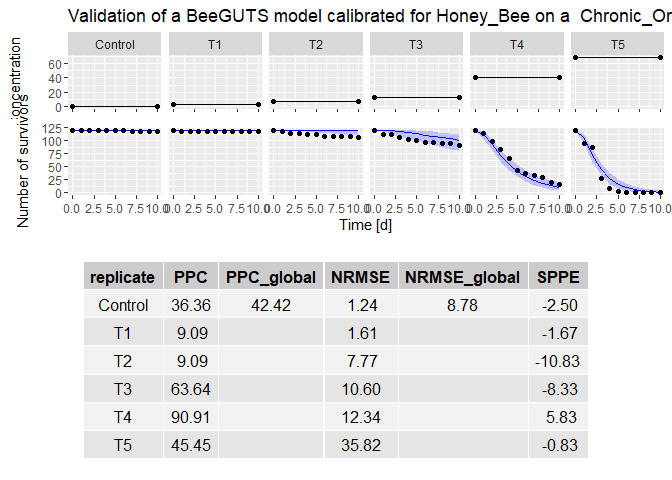
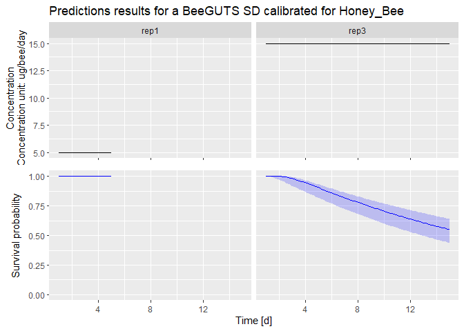
dataPredict <- data.frame(time = c(1:5, 1:15), conc = c(rep(5, 5), rep(15, 15)),  replicate = c(rep("rep1", 5), rep("rep3", 15))) # Prepare data for forwards prediction
prediction <- predict(fit, dataPredict) # Perform forwards prediction. At the moment, no concentration recalculation is performed in the forwards prediction. The concentrations are taken as in a chronic test
plot(prediction) # Plot of the prediction results