BayesMultiMode

BayesMultiMode is an R package for detecting and exploring multimodality using Bayesian techniques. The approach works in two stages. First, a mixture distribution is fitted on the data using a sparse finite mixture Markov chain Monte Carlo (SFM MCMC) algorithm. The number of mixture components does not have to be known; the size of the mixture is estimated endogenously through the SFM approach. Second, the modes of the estimated mixture in each MCMC draw are retrieved using algorithms specifically tailored for mode detection. These estimates are then used to construct posterior probabilities for the number of modes, their locations and uncertainties, providing a powerful tool for mode inference. See Basturk et al. (2023) and Cross et al. (2024) for more details.

Installing BayesMultiMode from CRAN

install.packages("BayesMultiMode")

Or installing the development version from GitHub

# install.packages("devtools") # if devtools is not installed 
devtools::install_github("paullabonne/BayesMultiMode")

Loading BayesMultiMode

library(BayesMultiMode)

BayesMultiMode for MCMC estimation and mode inference

BayesMultiMode provides a very flexible and efficient MCMC estimation approach : it handles mixtures with unknown number of components through the sparse finite mixture approach of Malsiner-Walli, Fruhwirth-Schnatter, and Grun (2016) and supports a comprehensive range of mixture distributions, both continuous and discrete.

Estimation

set.seed(123)

# retrieve galaxy data
y = galaxy

# estimation
bayesmix = bayes_fit(data = y,
                     K = 10,
                     dist = "normal",
                     nb_iter = 2000,
                     burnin = 1000,
                     print = F)

plot(bayesmix, draws = 200)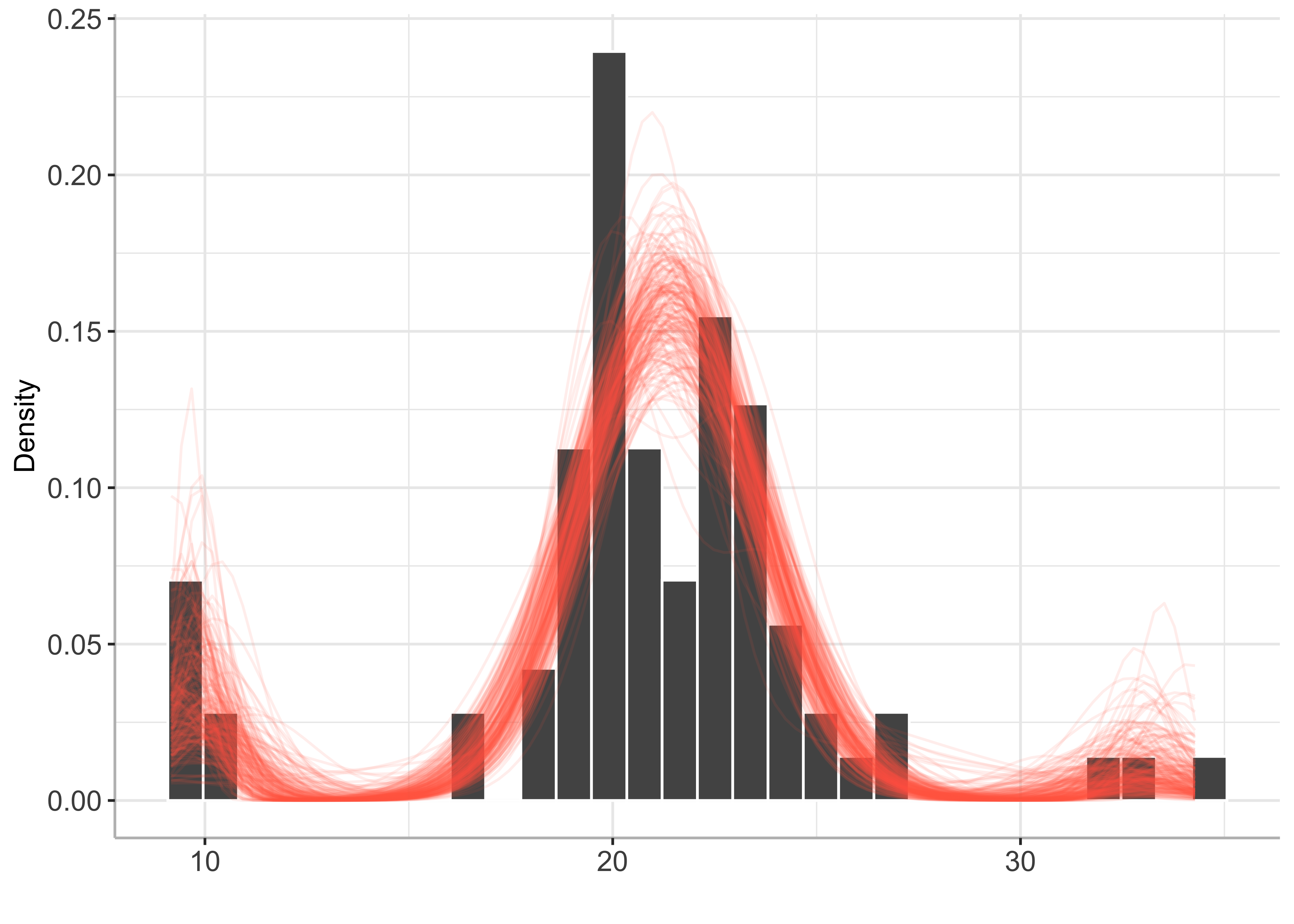

Mode inference

# mode estimation
bayesmode = bayes_mode(bayesmix)

plot(bayesmode)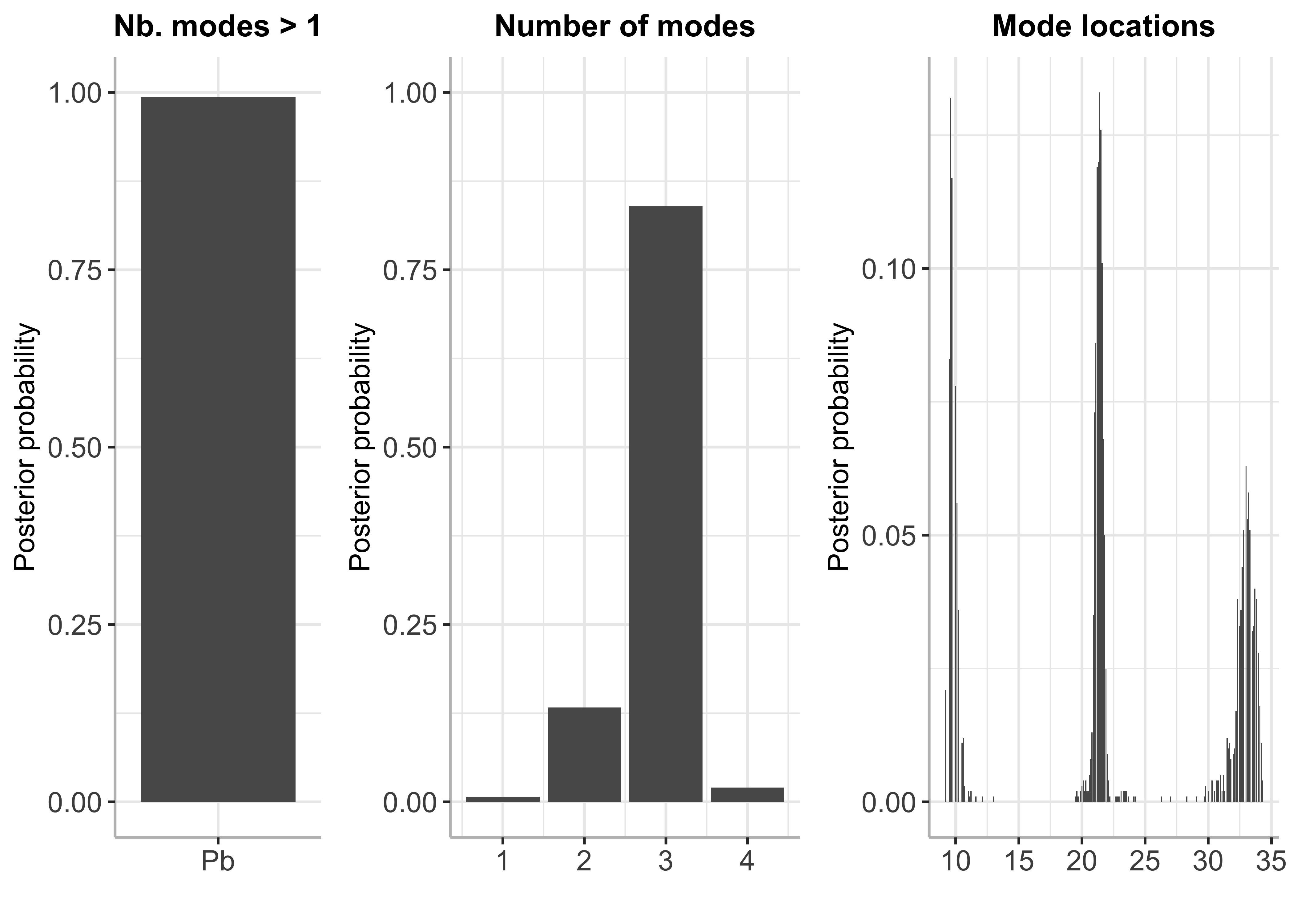

summary(bayesmode)

## Posterior probability of multimodality is 0.993 
## 
## Inference results on the number of modes:
##   p_nb_modes (matrix, dim 4x2): 
##      number of modes posterior probability
## [1,]               1                 0.007
## [2,]               2                 0.133
## [3,]               3                 0.840
## [4,]               4                 0.020
## 
## Inference results on mode locations:
##   p_loc (matrix, dim 252x2): 
##      mode location posterior probability
## [1,]           9.2                 0.021
## [2,]           9.3                 0.000
## [3,]           9.4                 0.000
## [4,]           9.5                 0.083
## [5,]           9.6                 0.132
## [6,]           9.7                 0.117
## ... (246 more rows)

BayesMultiMode for mode inference with external MCMC output

BayesMultiMode also works on MCMC output generated using external software. The function bayes_mixture() creates an object of class bayes_mixture which can then be used as input in the mode inference function bayes_mode(). Here is an example using cyclone intensity data (Knapp et al. 2018) and the BNPmix package for estimation. More examples can be found here.

library(BNPmix)
library(dplyr)

y = cyclone %>%
  filter(BASIN == "SI",
         SEASON > "1981") %>%
  dplyr::select(max_wind) %>%
  unlist()

## estimation
PY_result = PYdensity(y,
                      mcmc = list(niter = 2000,
                                  nburn = 1000,
                                  print_message = FALSE),
                      output = list(out_param = TRUE))

Transforming the output into a mcmc matrix with one column per variable

mcmc_py = list()

for (i in 1:length(PY_result$p)) {
  k = length(PY_result$p[[i]][, 1])
  
  draw = c(PY_result$p[[i]][, 1],
           PY_result$mean[[i]][, 1],
           sqrt(PY_result$sigma2[[i]][, 1]),
           i)
  
  names(draw)[1:k] = paste0("eta", 1:k)
  names(draw)[(k+1):(2*k)] = paste0("mu", 1:k)
  names(draw)[(2*k+1):(3*k)] = paste0("sigma", 1:k)
  names(draw)[3*k + 1] = "draw"
  
  mcmc_py[[i]] = draw
}

mcmc_py = as.matrix(bind_rows(mcmc_py))

Creating an object of class bayes_mixture

py_BayesMix = bayes_mixture(mcmc = mcmc_py,
                            data = y,
                            burnin = 0, # the burnin has already been discarded
                            dist = "normal",
                            vars_to_keep = c("eta", "mu", "sigma"))

Plotting the mixture

plot(py_BayesMix)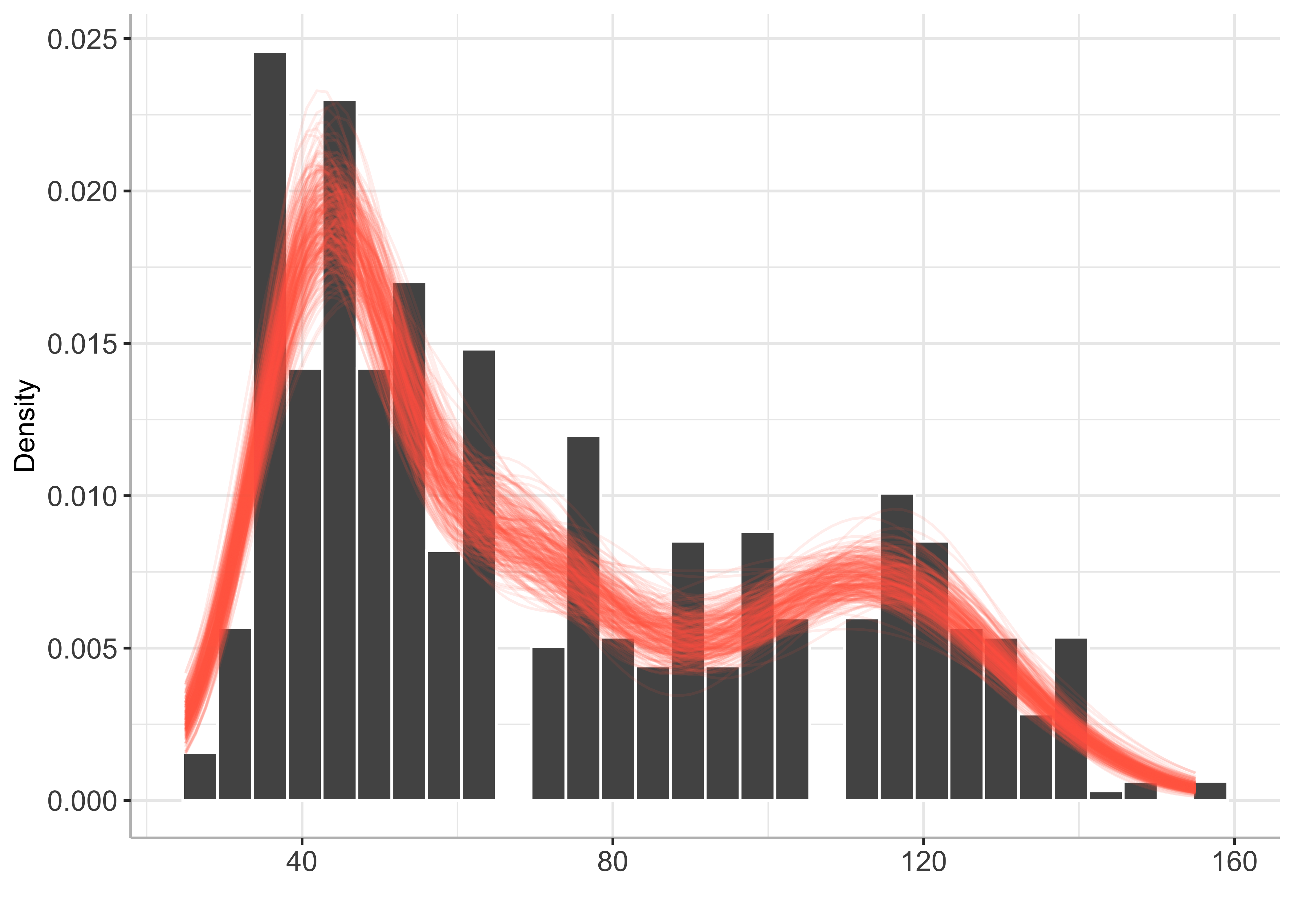

Mode inference

# mode estimation
bayesmode = bayes_mode(py_BayesMix)

# plot
plot(bayesmode)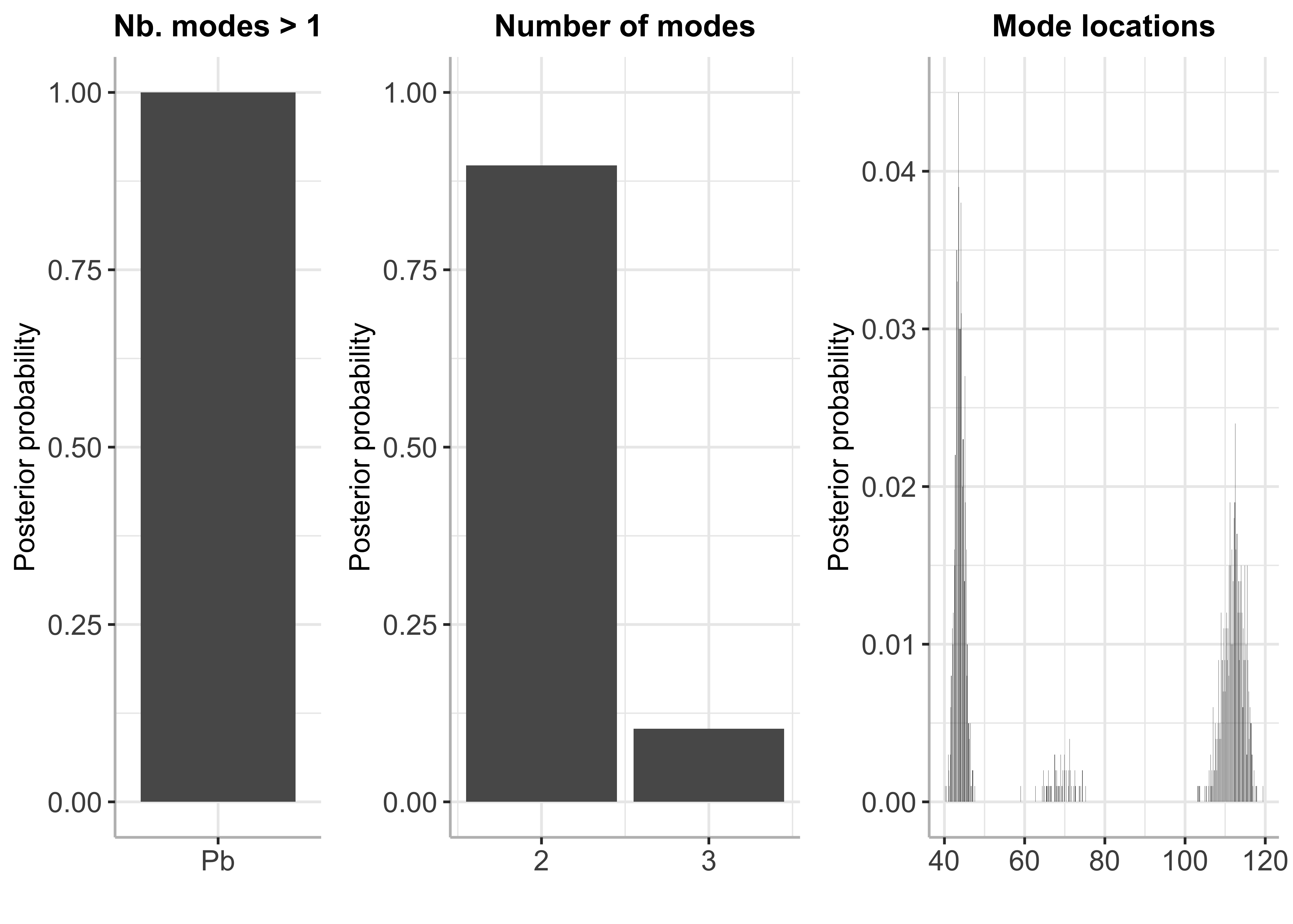

# Summary 
summary(bayesmode)

## Posterior probability of multimodality is 1 
## 
## Inference results on the number of modes:
##   p_nb_modes (matrix, dim 2x2): 
##      number of modes posterior probability
## [1,]               2                 0.897
## [2,]               3                 0.103
## 
## Inference results on mode locations:
##   p_loc (matrix, dim 793x2): 
##      mode location posterior probability
## [1,]          40.2                 0.001
## [2,]          40.3                 0.000
## [3,]          40.4                 0.000
## [4,]          40.5                 0.001
## [5,]          40.6                 0.000
## [6,]          40.7                 0.000
## ... (787 more rows)

BayesMultiMode for mode estimation in mixtures estimated with ML

It is possible to use BayesMultiMode to find modes in mixtures estimated using maximum likelihood and the EM algorithm. Below is an example using the popular package mclust. More examples can be found here.

set.seed(123)
library(mclust)

y = cyclone %>%
  filter(BASIN == "SI",
         SEASON > "1981") %>%
  dplyr::select(max_wind) %>%
  unlist()

fit = Mclust(y)

pars = c(eta = fit$parameters$pro,
         mu = fit$parameters$mean,
         sigma = sqrt(fit$parameters$variance$sigmasq))

mix = mixture(pars, dist = "normal", range = c(min(y), max(y))) # create new object of class Mixture
modes = mix_mode(mix) # estimate modes

plot(modes)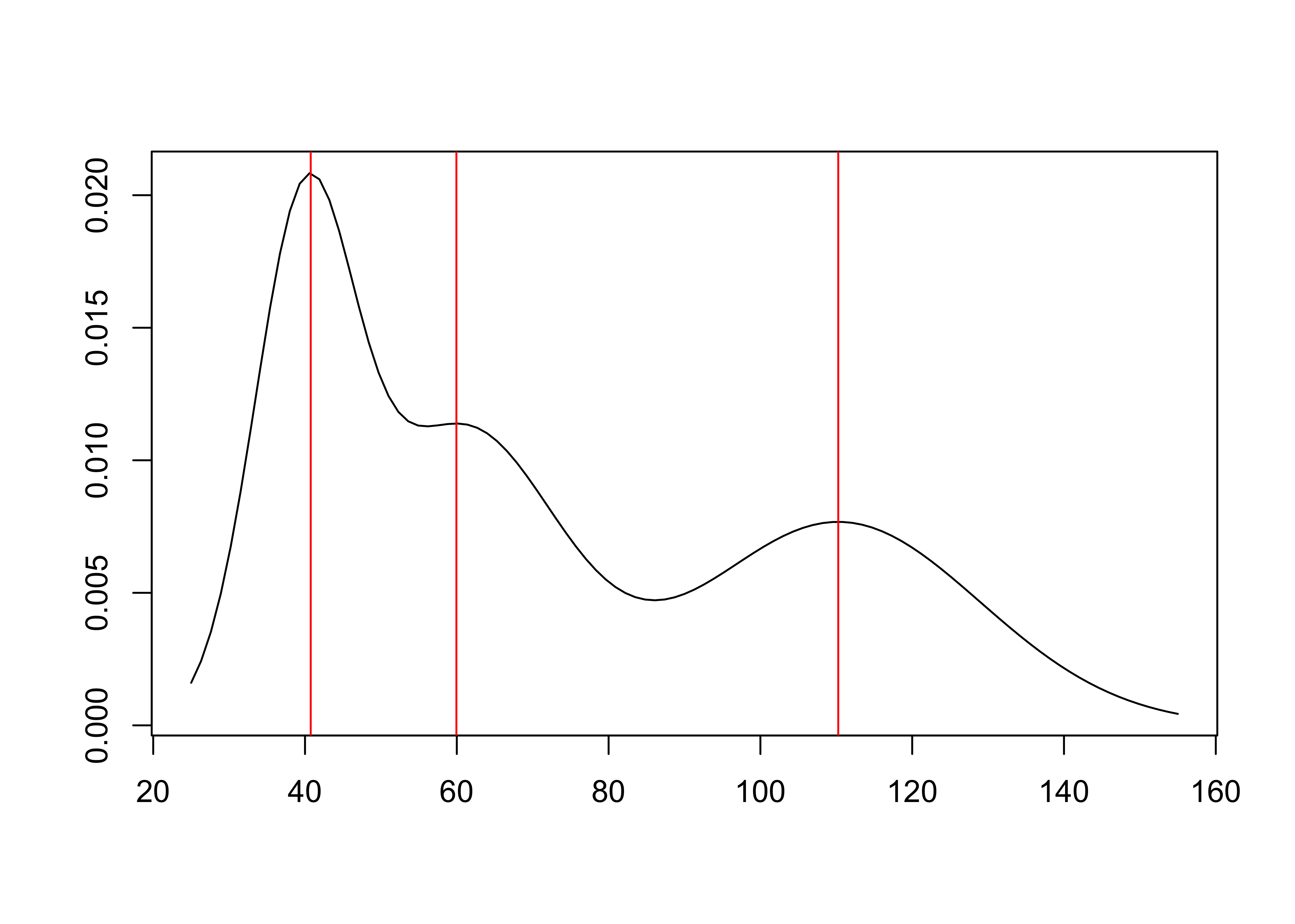

summary(modes)

## Modes of a normal mixture with 3 components.
## - Number of modes found: 3
## - Mode estimation technique: fixed-point algorithm
## - Estimates of mode locations:
##   mode_estimates (numeric vector, dim 3): 
## [1]  41  60 110

References