


![]()
Athlytics is a research-oriented R package for the longitudinal analysis of endurance training. It operates entirely on local Strava exports (or FIT/TCX/GPX files), avoiding API dependencies to ensure privacy and long-term reproducibility.
What is Strava? Strava is a popular fitness tracking platform used by millions of athletes worldwide to record and analyze their running, cycling, and other endurance activities. Users can export their complete activity history for offline analysis.
The package standardizes the workflow from data ingestion and quality control to model estimation and uncertainty quantification. Implemented endpoints include acute-to-chronic workload ratio (ACWR), aerobic efficiency (EF), and cardiovascular decoupling (pa:hr), alongside personal-best and exposure profiles suitable for single-subject and cohort designs. All functions return tidy data, facilitating statistical modeling and figure generation for academic reporting.
1. CRAN
install.packages("Athlytics")The source repository and development builds are linked from the package metadata for contributors.
Athlytics can parse TCX/GPX activity stream files when the suggested
xml2 package is installed. FIT support is
optional and uses FITfileR, which is available
from the FITfileR r-universe repository.
If your Strava export includes .fit files (and you want
Athlytics to parse them), install FITfileR:
install.packages(
  "FITfileR",
  repos = c("https://grimbough.r-universe.dev", "https://cloud.r-project.org")
)export_12345678.zip). As
of 1.0.5 the .zip can be passed directly
to load_local_activities(). Stream-based functions can
reuse that same ZIP path via export_dir:
calculate_pbs(), calculate_decoupling(), and
calculate_ef() when you want EF to use activity streams for
steady-state detection. calculate_ef() also falls back to
activity-summary averages when export_dir is omitted.
Unzipping into a directory is still supported and is a reasonable option
if you plan to iterate over the export many times.This example shows a common workflow: loading data for several athletes, calculating their training load, and comparing one athlete to the group average.
library(Athlytics)
library(dplyr)

# 1. Load data for a cohort of athletes, adding unique IDs
athlete1 <- load_local_activities("path/to/athlete1_export.zip") |> mutate(athlete_id = "A1")
athlete2 <- load_local_activities("path/to/athlete2_export.zip") |> mutate(athlete_id = "A2")
cohort_data <- bind_rows(athlete1, athlete2)

# 2. Calculate ACWR for each athlete in the cohort
cohort_acwr <- cohort_data |>
  group_by(athlete_id) |>
  group_modify(~ calculate_acwr(.x, activity_type = "Run", load_metric = "duration_mins")) |>
  ungroup()

# 3. Generate percentile bands to serve as a reference for the cohort
reference_bands <- calculate_cohort_reference(
  cohort_acwr,
  metric = "acwr_smooth",
  by = character(0),
  min_athletes = 2
)

# 4. Plot an individual's data against the cohort reference bands
individual_acwr <- cohort_acwr |> filter(athlete_id == "A1")
plot_with_reference(individual = individual_acwr, reference = reference_bands)All functions return clean, tidy tibble data frames,
making it easy to perform your own custom analysis or
visualizations.
Track how your training load is progressing to avoid ramping up too quickly — a key metric for monitoring training progression.
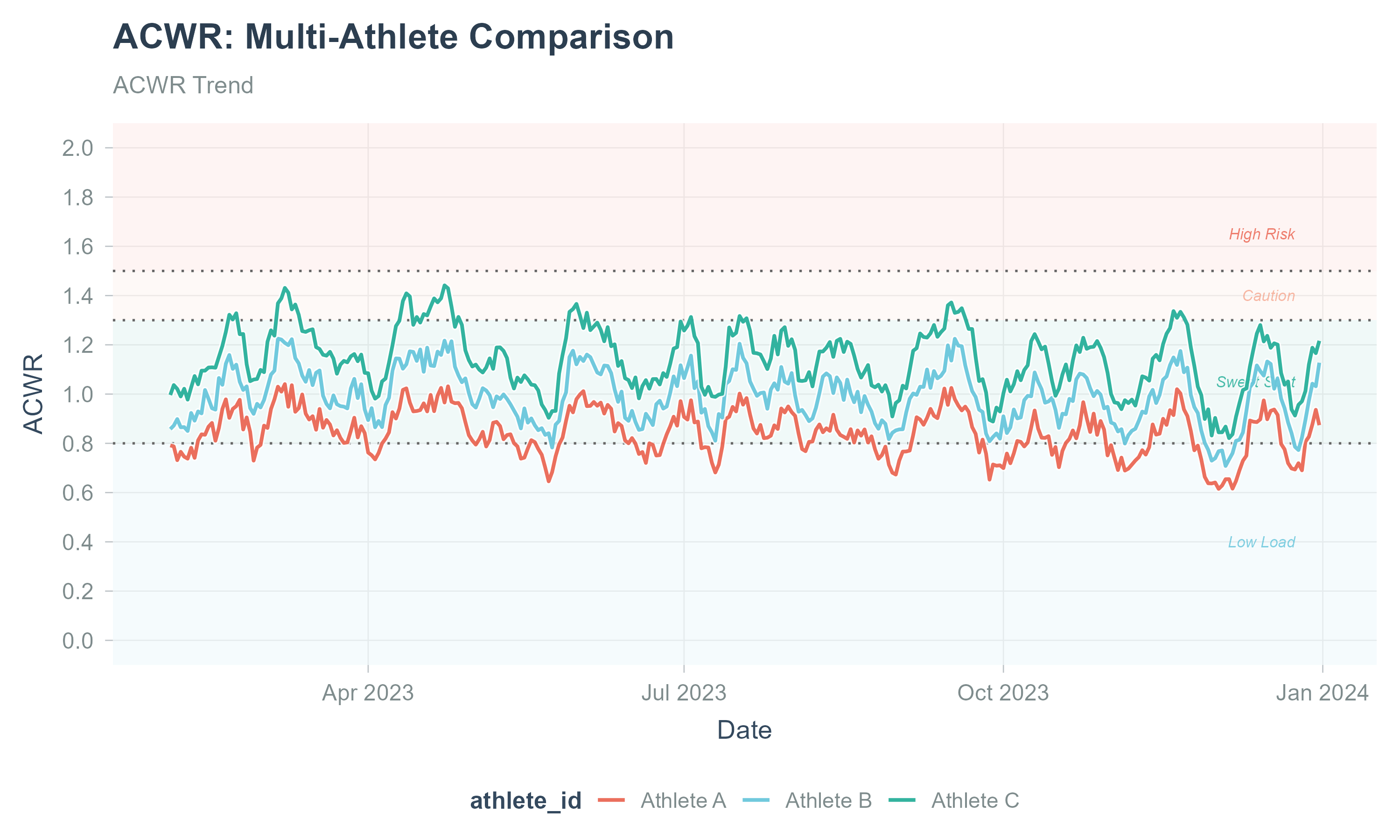
Learn more about ACWR analysis
See how your aerobic fitness is changing over time by comparing your output (speed or power) to your effort (heart rate). A rising trend is a great sign of improving fitness.
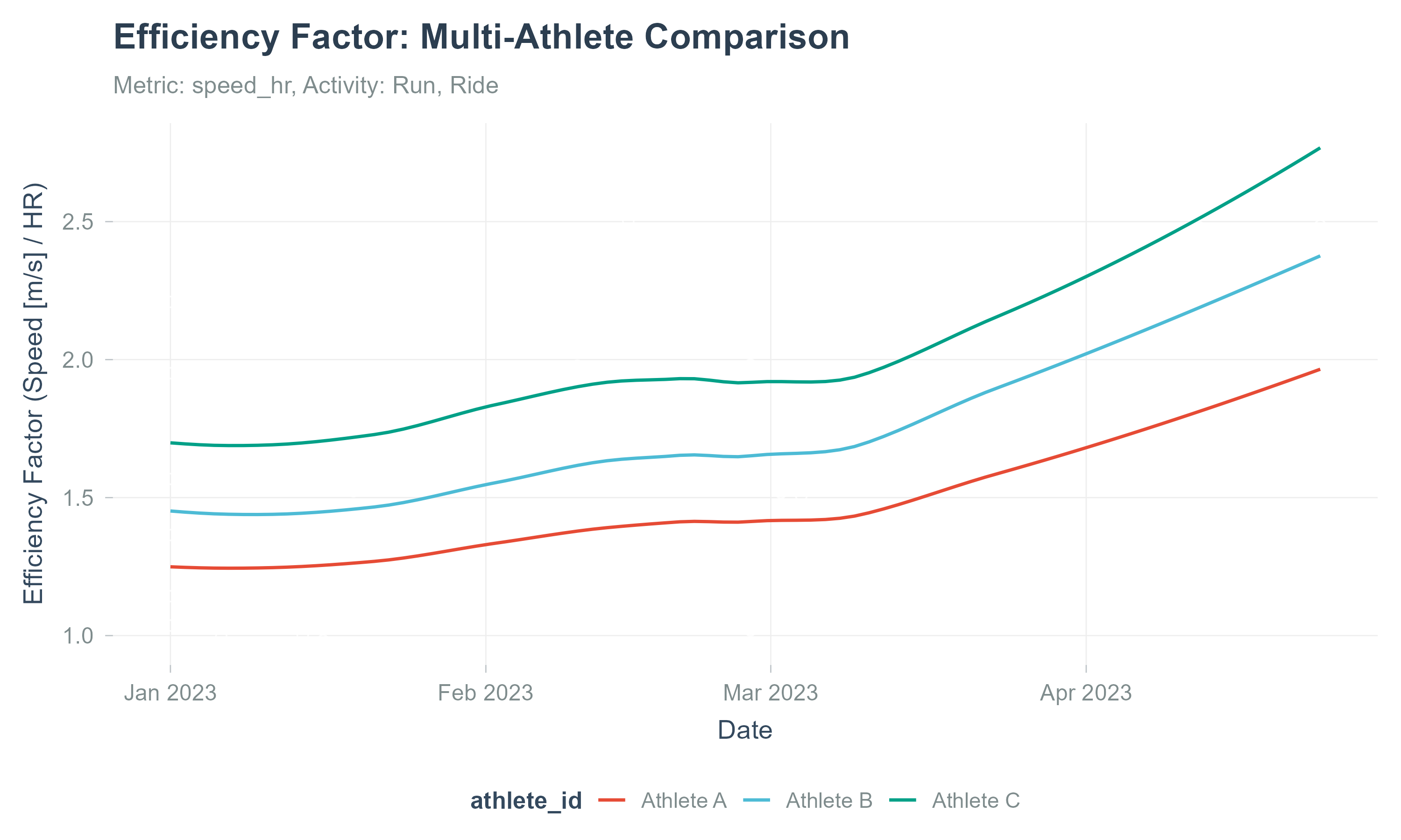
When an export ZIP or directory is supplied through
export_dir, EF uses activity streams for steady-state
detection; without it, EF is computed from activity-summary
averages.
Learn more about Aerobic Efficiency
Measure your endurance by analyzing how much your heart rate “drifts” upward during a steady-state workout. A low decoupling rate (<5%) is a marker of excellent aerobic conditioning.
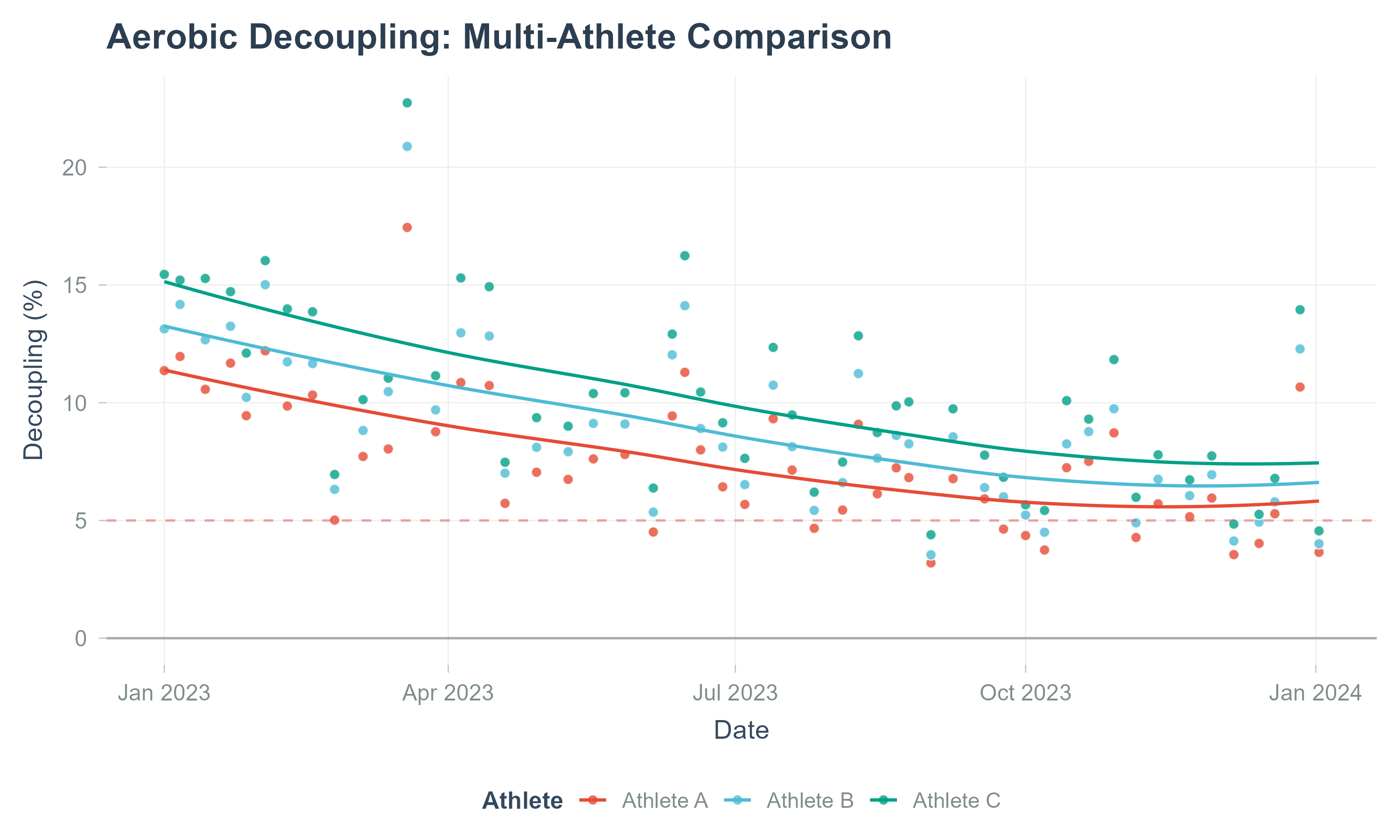
This release implements widely used constructs in endurance-exercise analytics: - ACWR: rolling acute (e.g., 7-day) vs chronic (e.g., 28-day) load ratios with smoothing options. - Aerobic Efficiency (EF): output (speed/power) relative to effort (heart rate) over time. - Cardiovascular Decoupling (pa:hr): drift between speed/power and heart rate during steady efforts.
Important: ACWR is a descriptive monitoring tool and should be interpreted with caution. It is not a validated injury-prediction model; see discussion in the sports science literature (e.g., DOI: 10.1007/s40279-020-01378-6).
We provide input validation, outlier handling, and activity-level QC filters (e.g., minimal duration, HR plausibility ranges). For cohort summarization, Athlytics computes percentile bands and supports stratification by sport, sex, or other covariates when available.
If you use Athlytics in academic work, please cite the software as well as the original methodological sources for specific metrics.
@software{athlytics2026,
  title   = {Athlytics: A Reproducible Framework for Endurance Data Analysis},
  author  = {Zhiang He},
  year    = {2026},
  version = {1.0.5},
  url     = {https://github.com/ropensci/Athlytics}
}Athlytics processes personal training records. Ensure appropriate consent for cohort analyses, de-identify outputs where required, and comply with local IRB/ethics and data-protection regulations.
Contributions are welcome! Please read our CONTRIBUTING.md guide. Please note that this package is released with a Contributor Code of Conduct. By contributing to this project, you agree to abide by its terms.
This package has been peer-reviewed by rOpenSci. We thank Eunseop Kim and Simon Nolte for their constructive reviews, and Prof. Benjamin S. Baumer and Prof. Iztok Fister Jr. for their valuable feedback and suggestions.